
03 / 05   Uniformity

Application note

Illumination, Shading, and Luminance Uniformity

Separate smooth field variation, fixed-pattern structure, and random noise before correcting them.

A uniform input should produce a predictable spatial output. For a camera, that means imaging a uniform radiance field; for a display, it means driving a uniform white or gray image. Smooth falloff, stripes, and localized patches can look similar in the result while arising from different physical mechanisms. A useful test separates those mechanisms before applying compensation.

Imaging: distinguish illumination from sensor response

Lens relative illumination compares image-plane irradiance across the field, commonly against the center:

RI(r)=Ei(r)Ei(0)RI(r)=\frac{E_i(r)}{E_i(0)}

Natural obliquity effects, pupil geometry, and mechanical vignetting can reduce peripheral illumination. A simple cos⁡4θ\cos^4\theta law is an idealized starting model, not a universal lens specification. Illumination nonuniformity and angle-dependent sensor response can further alter a captured flat field.

Photo-response nonuniformity (PRNU) describes spatial variation in light-response gain. Dark-signal nonuniformity (DSNU) describes spatial variation in the mean dark signal at a specified operating condition. Neither is simply another name for radial lens falloff. Row and column structure can contain offset and gain components; temporal noise varies between frames. Average repeated frames when estimating a stable spatial pattern.

Display: map emitted or reflected luminance

Drive a uniform field and measure luminance at defined locations and viewing angles. Backlight or emitter variation, optical films, projection geometry, and angular response can produce field variation. Localized nonuniformity is often called mura; its visibility depends on size, contrast, drive level, and surrounding content.

Measure more than one gray level when the application requires it. A map measured at full white does not characterize near-black mura or color-channel mismatch. Hold warm-up, drive settings, average picture level, and thermal conditions consistent. An imaging photometer captures dense spatial structure; a small set of spot ROIs can miss it.
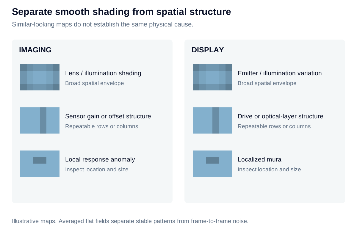
A camera flat field and a display uniform field can each contain smooth shading, row or column structure, and local defects, despite different causes.

View diagram at full size

State exactly what the uniformity number summarizes

For positive luminances measured over a declared ROI set, a common summary is:

Umin⁡/max⁡=100Lmin⁡Lmax⁡%U_{\min/\max}=100\frac{L_{\min}}{L_{\max}}\%

Also retain the mean, extrema, and spatial map. Nine, thirteen, or another number of points may be appropriate to a specified protocol; the count alone does not establish standard compliance. Use a uniform test image, not a contrast checkerboard. For an acquisition test, apply the same logic to a linear, dark-corrected flat-field signal while accounting for the uniformity of the reference source.
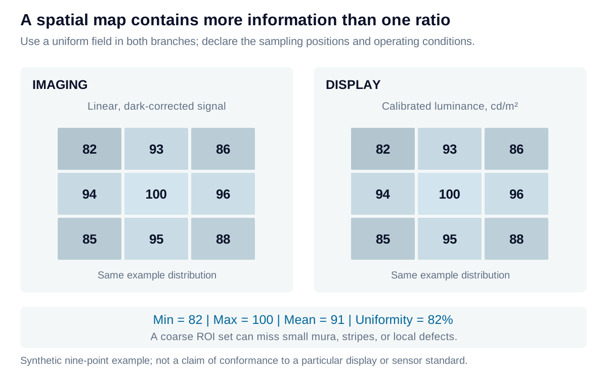
The same nine sample values can summarize a display luminance map or a linear camera flat field. Their min-to-max ratio is one summary, while the map preserves spatial information.

View diagram at full size

Correct the stable components without hiding limitations

A simple camera calibration uses dark frame D(x,y)D(x,y) and flat frame F(x,y)F(x,y) acquired under compatible conditions:

Icorr(x,y)=[I(x,y)−D(x,y)]F−D‾F(x,y)−D(x,y)I_{\mathrm{corr}}(x,y)=\big[I(x,y)-D(x,y)\big] \frac{\overline{F-D}}{F(x,y)-D(x,y)}

The denominator must be valid, positive, and unsaturated. The correction can remove repeatable offset and gain variation in that calibrated configuration; it cannot recover clipped information or eliminate random noise. Strong amplification in dark corners also amplifies uncertainty.

For a display, spatial drive correction adjusts the emitted pattern toward a target luminance. Its calibration belongs to the selected gray level, channel, angle, and thermal state; limited headroom may require reducing the target brightness. In both branches, verify residual nonuniformity with independent captures and representative operating conditions.

Iris Optics can help diagnose camera shading and display mura, design defensible spatial measurements, and validate compensation without confusing a corrected map with recovered signal quality.

Explore the model

Nine-point luminance uniformity

Enter a 3 × 3 set of display luminances or calibrated image-plane readings under a defined uniform field.

Change the values to update the results and visualization.

Minimum / maximum uniformity
89 %
Mean luminance
186.78 cd/m²
Minimum luminance
178 cd/m²
Maximum luminance
200 cd/m²
Nine-ROI coefficient of variation
3.5851 %

Read the map top-to-bottom, left-to-right. It shows the supplied locations only; no spatial interpolation or defect detection is implied.

Nine-point luminance uniformity: normalized mapTop row, middle row, bottom row: 180, 190, 182, 192, 200, 190, 178, 188, 181 cd/m². Tile brightness is normalized to the highest reading.ROI 1180ROI 2190ROI 3182ROI 4192ROI 5200ROI 6190ROI 7178ROI 8188ROI 9181
Luminance in cd/m²; illustrative normalized grayscale, not a physical display simulation.
Formula & assumptions

U = Lmin/Lmax; CV = population standard deviation / mean, over these nine readings.

A user-defined nine-point sampling example, not an ANSI/ICDM compliance test. Locations, ROI sizes, pattern, temperature, integration time and exposure must be controlled. Sparse readings can miss mura, local defects and row/column structure. The map is normalized to the brightest input; it is not a calibrated reproduction of visible brightness. These ROI statistics do not measure sensor PRNU or DSNU.

Explore the model

Dark and flat-field correction

Calculate one imaging pixel’s offset and gain correction from matching dark and uniform-field references.

Change the values to update the results and visualization.

Gain correction
1.25 ×
Dark-subtracted signal
500 DN
Corrected signal, no offset
625 DN

Large gains also amplify noise. A valid denominator does not guarantee a useful calibration; weak flat signals and unstable pixels need separate handling.

Dark and flat-field correction: interactive plotLinear signal / DN against Stage: raw (0), subtract (1), scale (2). Correction stages.0-62.50.487.50.82381.23881.65382688Stage: raw (0), subtract (1), scale (2)Linear signal / DN
Correction stages
Formula & assumptions

g = (Fref − Dref)/(F − D); corrected signal = (R − D)g.

A scalar camera correction at the same gain, exposure, temperature, spectrum and optical configuration. Reference terms may represent a chosen normalizing region. No offset is re-added; a negative result is retained. Saturation, unstable defects, stray light and temporal noise cannot be recovered this way. Display compensation also needs calibrated transfer functions and headroom; this formula alone is not a display correction map.

From estimate to application

Separate the device from the measurement setup.

Iris Optics can help characterize illumination, camera response, and display output, then develop calibration and acceptance tests around the variation that matters.

Discuss uniformity and calibration