
Fine detail can disappear before it becomes too small to count in pixels. The relevant question is how much modulation remains at its spatial frequency. A camera transfers a scene pattern into an image; a display transfers image data into a visible pattern. Both paths include optics, sampling, and processing that influence the measured response.
Distinguish square-wave and sinusoidal tests
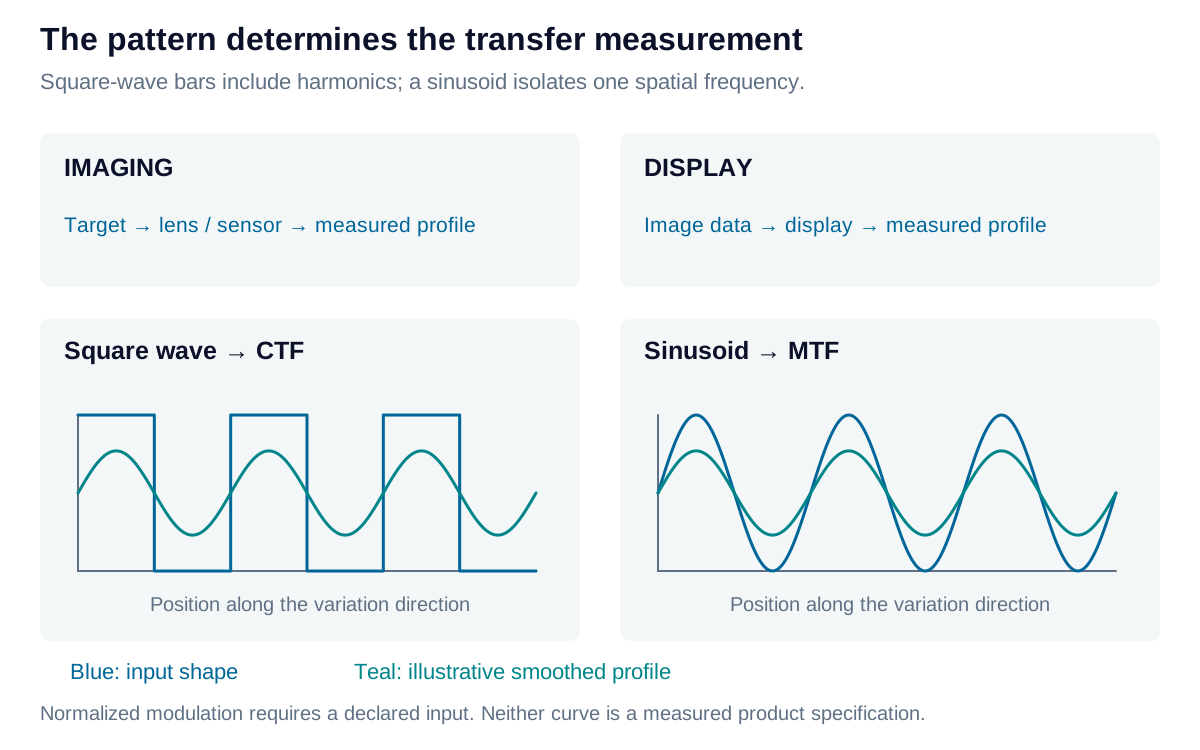
A black-and-white bar pattern contains a fundamental frequency and odd harmonics. Its measured Michelson modulation is:
When reporting a normalized contrast transfer function, state the input modulation:
For a linear, shift-invariant system, MTF describes sinusoidal modulation transfer. CTF measures a square-wave response; they are related through the harmonics but are not interchangeable curves. A bar-pattern percentage is modulation, not the white-to-black luminance ratio.
Imaging: characterize the complete acquisition condition
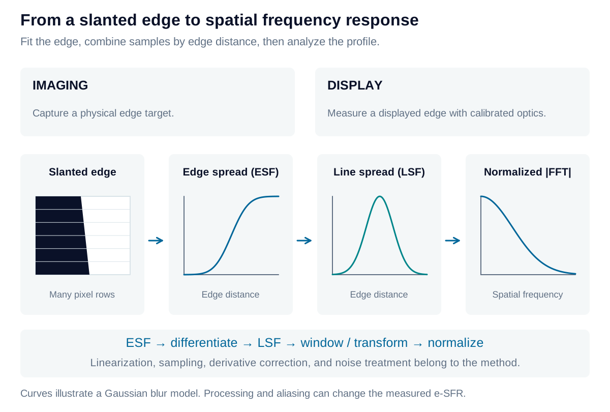
Measure a calibrated target at the required working distance, aperture, focus, illumination spectrum, and exposure. A slanted-edge method estimates an oversampled edge spread function from many pixel rows. Differentiating it gives the line spread function; the normalized magnitude of its Fourier transform gives an edge-based spatial frequency response, or e-SFR.
The edge must be linearized using the camera’s response. Edge fitting, binning, windowing, differentiation correction, and noise handling affect the estimate. Sharpening can produce values above unity; this processed response is not a lens-only MTF. Record raw versus processed output and report the field positions actually tested.
Display: characterize the pattern and the observer path
Measure physical luminance profiles of displayed bars, sinusoids, or edges at the intended viewing geometry. The measuring camera’s own lens and sensor can limit the result. Control display scaling, pixel phase, subpixel structure, drive level, and enhancement; characterize instrument response. For near-eye displays, specify the measurement entrance-pupil size and position, virtual-image focus, and angular calibration.
Bar-pattern CTF is a useful display test when its frequency and phase are specified. Display MTF is also meaningful with an appropriate method. Both displays and cameras are sampled systems: aliasing and phase sensitivity are reasons to qualify the procedure, not a universal reason to prefer one metric for an entire device class.
Specify scale, field, and direction
One line pair is one spatial cycle. Use lp/mm in a named object, image, or display plane, or cycles/degree at a specified viewing distance. For pitch in mm, the one-dimensional sampling limit is:
This Nyquist frequency does not guarantee faithful detail near the limit. Target and measurement sampling, optical filtering, and orientation all matter. Record both horizontal and vertical variation directions: vertical bars vary horizontally.
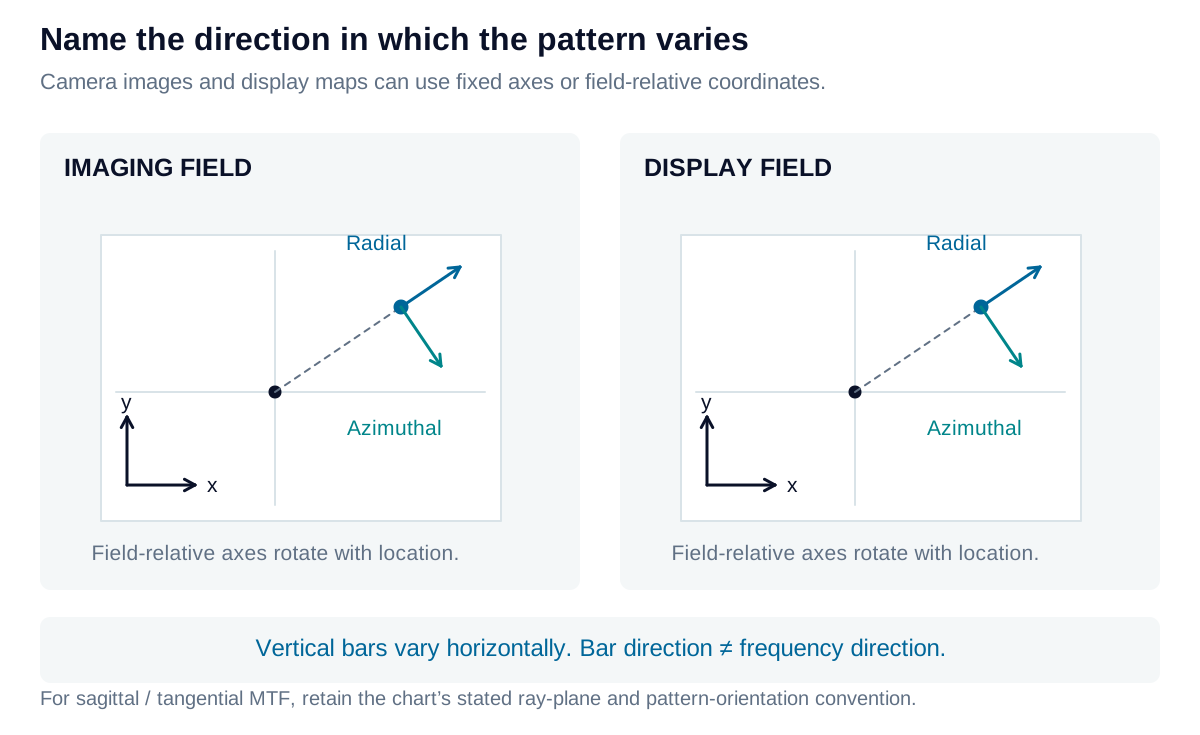
Lens data often use sagittal and tangential sections tied to the optical axis and field point. State whether a label describes the ray plane, line orientation, or frequency direction before comparing it with a horizontal/vertical test. A center-and-corner map may be sufficient for one task; a denser field grid may be necessary for another. No single ROI count defines a complete characterization.
Reading sagittal and tangential directions
At an off-axis field point, the meridional or tangential plane contains the optical axis and the chief ray. The sagittal plane is perpendicular to it and also contains the chief ray. These ray-plane definitions describe the optical geometry.
Many lens MTF charts label radially oriented line structures as sagittal and structures tangent to a field circle as tangential or meridional. Their intensity variation is perpendicular to the lines: radial bars vary in the azimuthal direction, and tangential bars vary radially. A label for line orientation is therefore not the same as a label for frequency direction.
Retain the manufacturer’s convention when reading a published curve. For a measured camera or display map, recording the actual pattern orientation and variation direction removes the ambiguity. Away from the field center, these local directions generally do not coincide with fixed horizontal and vertical axes.
Iris Optics can develop acquisition and display resolution tests that separate device performance from target, sampling, and instrument limits, with acceptance criteria matched to the intended detail.