
05 / 06   Spectral transfer

Application note

Source, Material, and Observer

Build a color calculation from a measured spectrum and clearly defined weighting functions.

A useful spectral model keeps the illumination, sample, and observer separate. This allows one measured material spectrum to be evaluated under different sources without confusing a change in lighting with a change in the material. The separation is valid only while the measurement geometry and physical operating conditions remain applicable.

Define the three factors

Let S(λ)S(\lambda) describe the incident spectral distribution and H(λ)H(\lambda) the sample’s spectral power throughput. In a simple transmission model, H=TH=T; in a compatible reflectance measurement, HH represents the measured reflection quantity. For a linear, nonfluorescent response:

C(λ)=S(λ)H(λ)C(\lambda)=S(\lambda)H(\lambda)

Here HH acts on spectral power, not the complex electric-field amplitude used in coherent-wave transfer functions. A passive transmitted or collected-power fraction lies between zero and one. Reflectance factors defined relative to a reference geometry need their own interpretation and are not universally bounded by one.
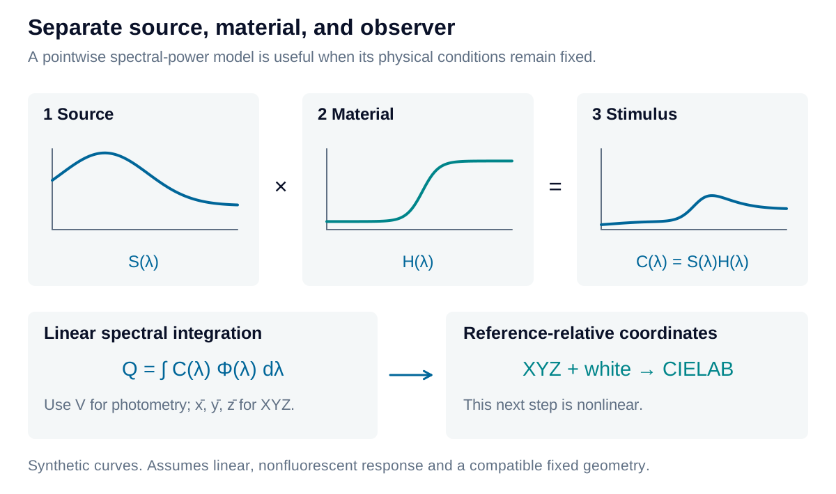
A source spectrum is multiplied by a material throughput curve; the resulting stimulus is then integrated against observer functions.

View diagram at full size

The observer is represented by a weighting function Φ\Phi or by three color-matching functions. A scalar channel has response:

Q=∫S(λ)H(λ)Φ(λ) dλQ=\int S(\lambda)H(\lambda)\Phi(\lambda)\,d\lambda

This integral is linear in the stimulus. It is not a complete model of perceived appearance: adaptation, spatial context, and subsequent nonlinear processing are absent.

Normalize a luminous ratio

Compare the filtered and unobstructed source using the same wavelength limits and photopic weighting:

ηv=∫S(λ)H(λ)V(λ) dλ∫S(λ)V(λ) dλ\eta_v=\frac{\int S(\lambda)H(\lambda)V(\lambda)\,d\lambda} {\int S(\lambda)V(\lambda)\,d\lambda}

The ratio expresses the retained luminous contribution in the defined geometry; multiply by 100 for percent. A neutral throughput H=0.40H=0.40 gives 40% for any source with a positive denominator. A selective filter generally gives different results under different sources, even when its measured throughput curve is unchanged.

Preserve one common XYZ scale

For relative object colorimetry, define the reference as H=1H=1 and normalize its YY to 100:

k=100∫S(λ)yˉ(λ) dλ,(X,Y,Z)=k∫SH (xˉ,yˉ,zˉ) dλk=\frac{100}{\int S(\lambda)\bar y(\lambda)\,d\lambda},\qquad (X,Y,Z)=k\int SH\,(\bar x,\bar y,\bar z)\,d\lambda

The same kk multiplies all three integrals. Independently normalizing X, Y, and Z would change the coordinate system. For the CIE 1931 observer, yˉ=V\bar y=V and Y/100Y/100 equals the luminous ratio over matching limits.
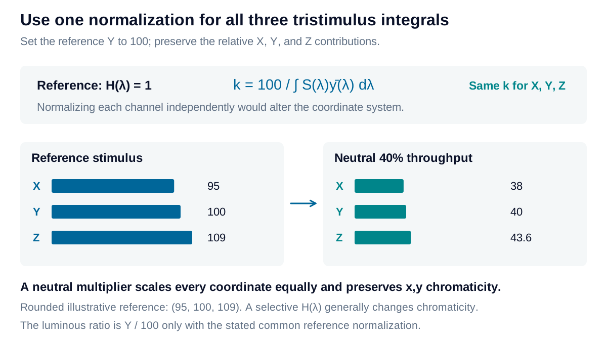
The same neutral throughput preserves source chromaticity while a selective throughput changes relative XYZ contributions. A common normalization sets only the reference Y to 100.

View diagram at full size

D65 supplies a defined daylight spectral distribution. The standard 2° and 10° observers represent different color-matching field conditions; they are not a general switch between central and peripheral vision. Keep the illuminant, observer, wavelength coverage, and reference white attached to every result.

Identify where the cascade stops applying

Angle, polarization, temperature, sample condition, and collection geometry can alter HH. Interchanging sources is useful when those conditions stay fixed and the sample response remains linear. Fluorescence requires coupling excitation wavelengths to emission wavelengths; a single pointwise multiplier cannot describe that conversion.

Measured spectra must also resolve important source and filter structure. Align the wavelength grids, use compatible units, and integrate with the actual interval widths. Missing spectral tails are missing evidence, not demonstrated zeros. The calculator uses an explicitly synthetic passive throughput curve to show the framework; an application decision needs representative measured data and its uncertainty.

Explore the model

Source–material–observer explorer

Change a simple material spectrum and inspect the resulting stimulus and observer-weighted response.

Change the values to update the results and visualization.

D65: standard daylight. E: equal spectral power per nm.

Wavelength-interval mean
55.745 %
V-only weighted mean
55.157 %
D65-weighted luminous throughput
53.16 %
XYZ · white Y = 100
60.845, 53.16, 21.855
CIELAB · same illuminant white
77.97, 25.88, 44.916

The source and stimulus share one scale; material throughput is a fraction. In the observer-weighted plot, the unfiltered reference integrates to 100 and the sample integrates to its luminous throughput percentage. Changing the source changes these results while H stays fixed.

Source–material–observer explorer: interactive plotRelative spectral value against Wavelength in standard air / nm. Curves: Source S / peak(S); Material H; Stimulus SH / peak(S). 36004540.25480.46420.67360.88301Wavelength in standard air / nmRelative spectral value
Source S / peak(S)Material HStimulus SH / peak(S)
Source–material–observer explorer — observer weighting: interactive plotY contribution / (% per nm) against Wavelength in standard air / nm. Curves: Unfiltered source × observer; Source × material × observer. 36004540.2165480.4316420.6477360.8628301.08Wavelength in standard air / nmY contribution / (% per nm)
Unfiltered source × observerSource × material × observer
Formula & assumptions

C(λ) = S(λ)H(λ); (X,Y,Z) = k ∫ C(λ)(x̄,ȳ,z̄)dλ; k = 100/∫S(λ)ȳ(λ)dλ.

Synthetic passive power throughput, fixed geometry and polarization, no wavelength conversion. A 5 nm linear transition joins two flat bands. Integration uses the full 360–830 nm, 1 nm standard-air wavelength grid and trapezoidal quadrature. Lab uses the same grid, illuminant, and perfect-throughput white. This is a teaching model, not uploaded measurement data.

Reference data: CIE 1931 2° observer and Illuminant D65. Numeric tables © CIE, used under CC BY-SA 4.0; derived data plots share this license. Tables retained at 1 nm on the common 360–830 nm interval. Figures and calculations by Iris Optics.

From estimate to application

Build a measurement model around your application.

Share your spectra and measurement geometry. Iris Optics can help identify the source, material, and detector assumptions needed for a useful result.

Discuss your spectral analysis