Spectral Averages and Color Difference

A single average cannot describe every useful property of an optical spectrum. A coating can retain substantial radiant power while suppressing visually important wavelengths, or preserve luminance while shifting color. Start by specifying the quantity that the acceptance criterion is meant to control.

Choose what receives equal weight

For a throughput curve $H$ over $[\lambda_a,\lambda_b]$ , a uniform-in-wavelength mean is:

\bar H_\lambda=\frac{\int_{\lambda_a}^{\lambda_b}H(\lambda)\,d\lambda} {\lambda_b-\lambda_a}

This gives equal weight to equal wavelength intervals. It is not generally the arithmetic mean of measured rows. Dense sampling in one band must not give that band extra weight simply because more measurements were taken there.

Photopic-only and source-weighted luminous means instead use:

\bar H_V=\frac{\int HV\,d\lambda}{\int V\,d\lambda},\qquad \bar H_{SV}=\frac{\int SHV\,d\lambda}{\int SV\,d\lambda}

The V-only result corresponds to an equal-energy spectral source over the integration band. It is not automatically the luminous result under daylight or a particular lamp. State the wavelength interval and source with every reported percentage.

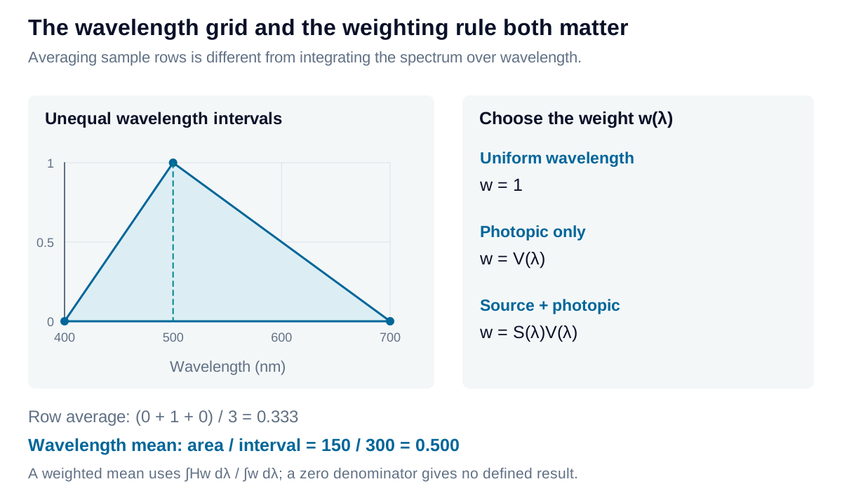
Uniform, photopic-only, and source-weighted means assign different importance to a synthetic throughput spectrum. Irregular sample spacing changes integration weights.

View diagram at full size

Integrate irregular samples with interval widths

For ordered samples of an integrand $f_i=f(\lambda_i)$ , trapezoidal quadrature gives:

\int f(\lambda)\,d\lambda\approx \sum_{i=0}^{N-2}\frac{f_i+f_{i+1}}{2}(\lambda_{i+1}-\lambda_i)

For example, throughput values $(0,1,0)$ sampled at wavelengths $(400,500,700)$ nm have an arithmetic row mean of $1/3$ . Their piecewise-linear integral is 150 nm, giving a wavelength mean of $150/300=0.5$ . Sampling density and interval width are different quantities.

Apply the rule separately to a weighted numerator and denominator on a compatible grid. Interpolation aligns data; it cannot recover narrow spectral features that were never measured. Even a uniform grid requires consistent endpoint treatment.

Carry XYZ into a reference-relative space

CIELAB expresses XYZ relative to a white reference $(X_n,Y_n,Z_n)$ computed using the same illuminant and observer:

L^*=116f(Y/Y_n)-16

a^*=500[f(X/X_n)-f(Y/Y_n)],\qquad b^*=200[f(Y/Y_n)-f(Z/Z_n)]

Lightness $L^*$ is nonlinear in relative Y. The $a^*$ and $b^*$ coordinates describe opposing chromatic directions. Lab therefore does not preserve the additive spectral relationship used to calculate XYZ.

The CIELAB piecewise function

With $\delta=6/29$ :

f(t)=\begin{cases} t^{1/3},&t>\delta^3\\ t/(3\delta^2)+4/29,&t\leq\delta^3 \end{cases}

The linear branch makes the transformation finite near zero and joins the cube-root branch continuously in value and slope. The sample and reference XYZ must use the same normalization. A perfect reference has $(L^*,a^*,b^*)=(100,0,0)$ ; zero XYZ gives $(0,0,0)$ .

For a spectrally neutral 40% sample with the same reference white, the common XYZ scale cancels in the ratios: $L^*\approx69.47$ and $a^*=b^*=0$ . By contrast, two selective samples can have the same wavelength-average throughput while returning different Lab coordinates. A scalar throughput specification and a color specification therefore answer different questions.

Compare colors with a named metric

CIE76 is Euclidean distance in Lab:

\Delta E_{76}=\sqrt{(\Delta L^*)^2+(\Delta a^*)^2+(\Delta b^*)^2}

CIEDE2000, written $\Delta E_{00}$ , adjusts lightness, chroma, and hue contributions and includes a chroma–hue interaction. It is a different metric, not another way to compute the same numerical distance. Its standard parametric factors are commonly set to one; application-specific conditions may require an agreed alternative.

The structure of the CIEDE2000 calculation

Define the normalized lightness, chroma, and hue contributions using the CIEDE2000 corrections:

q_L=\frac{\Delta L'}{k_LS_L},\qquad q_C=\frac{\Delta C'}{k_CS_C},\qquad q_H=\frac{\Delta H'}{k_HS_H}

Then:

\Delta E_{00}=\sqrt{q_L^2+q_C^2+q_H^2+R_Tq_Cq_H}

The primed differences, scale terms $S_L,S_C,S_H$ , and rotation term $R_T$ follow the full CIEDE2000 definition. They are not obtained by directly substituting $\Delta a^*$ and $\Delta b^*$ . In particular, hue wraps around a circle and becomes undefined at zero chroma, requiring explicit branch handling. The calculator implements those branches and uses $k_L=k_C=k_H=1$ .

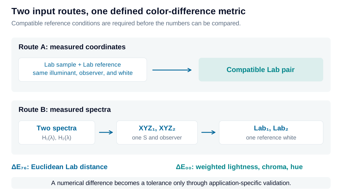
Two routes reach the same color-difference calculation: enter compatible Lab coordinates directly, or derive them from two spectra under the same illuminant, observer, and white reference.

View diagram at full size

There are two useful input routes to $\Delta E_{00}$ : compare compatible measured Lab coordinates, or calculate XYZ and Lab from each spectrum first. The latter preserves the ability to investigate source-dependent differences. Both routes require matching reference conditions; entering Lab alone cannot verify them.

A difference value is not a universal pass/fail decision. Geometry, texture, gloss, adaptation, measurement variation, and the task affect visibility and acceptability. Establish a tolerance using representative parts and controlled viewing, then confirm that the measurement can resolve that tolerance.

Spectral Averages and Color Difference

Choose what receives equal weight

Carry XYZ into a reference-relative space

Compare colors with a named metric

Compare spectral averages

Compare two CIELAB measurements

Make optical acceptance criteria reproducible.