02 / 06   Color coordinates

Application note

From Spectra to Color Coordinates

Connect spectral distributions, three-channel measurements, and the chromaticity diagram.

A measured spectrum may contain hundreds of wavelength samples. A colorimetric observer reduces that information to three coordinates. This reduction supports reproducible color matching, but it cannot preserve the full spectrum or every aspect of appearance. Choosing the right representation makes those limits visible.

Project a spectrum into three dimensions

LMS coordinates describe responses using a specified set of cone fundamentals. CIE XYZ uses standardized color-matching functions xˉ,yˉ,zˉ\bar x,\bar y,\bar z. For a spectral stimulus PλP_\lambda:

[XYZ]=k∫Pλ(λ)[xˉ(λ)yˉ(λ)zˉ(λ)] dλ\begin{bmatrix}X\\Y\\Z\end{bmatrix} =k\int P_\lambda(\lambda) \begin{bmatrix}\bar x(\lambda)\\\bar y(\lambda)\\\bar z(\lambda)\end{bmatrix}\,d\lambda

The common factor kk sets the scale. The CIE 1931 observer assigns photopic luminance information to YY; XX and ZZ are not separate cone signals. A matrix conversion between color coordinates requires compatible observer definitions. Arbitrary Gaussian LMS curves cannot be transformed into exact CIE 1931 XYZ values by a universal matrix.
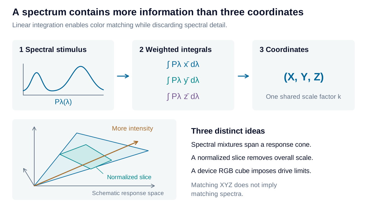
An input spectrum is integrated against three sensitivity functions, producing three coordinates; different spectra can produce matching coordinates.

View diagram at full size

For a monochromatic stimulus with fixed radiant power, changing wavelength traces a parametric curve in response space. Increasing its power moves outward along a ray from the origin. Mixtures add the response vectors. Without a power limit, nonnegative spectra generate a convex cone of accessible responses, rather than filling a bounded cube.

Some mathematical coordinates remain inaccessible: a stimulus cannot excite only M cones while producing exactly zero L response where their sensitivities overlap. This restriction concerns ordinary spectral stimulation, not unusual adaptation experiments. The familiar unit RGB cube instead describes the limited drive range of a specified three-primary system.

Remove the overall scale

Chromaticity divides each tristimulus value by their sum:

x=XX+Y+Z,y=YX+Y+Z,z=1−x−yx=\frac{X}{X+Y+Z},\qquad y=\frac{Y}{X+Y+Z},\qquad z=1-x-y

This maps a three-dimensional ray to the plane x+y+z=1x+y+z=1. The two independent coordinates x,yx,y retain chromaticity while discarding magnitude. Add YY to form xyYxyY when luminance information is needed. At X=Y=Z=0X=Y=Z=0, chromaticity is undefined.

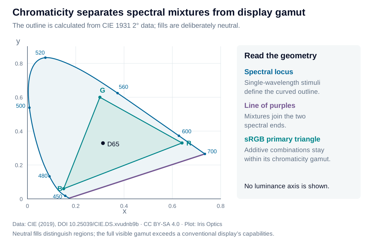
The CIE 1931 chromaticity diagram distinguishes the spectral locus, the line of purples, and the smaller triangle spanned by the sRGB primaries.

View diagram at full size

Plot data: CIE (2019), CC BY-SA 4.0. Diagram adapted by Iris Optics under the same license.

The curved spectral locus represents single wavelengths. The straight closing edge joins the extreme spectral ends through purple mixtures. Three non-collinear display primaries span a triangle inside the accessible chromaticity region. A larger triangle does not imply more brightness or more distinguishable code values.

Mix in a linear space

Two additive stimuli mix on the line joining their chromaticities, but equal radiant powers do not generally place the result at the midpoint. First add XYZ, then normalize. The chromaticity weights depend on each stimulus’s X+Y+ZX+Y+Z contribution.

Why additive mixtures lie on a straight chromaticity line

Let CA=(XA,YA,ZA)\mathbf C_A=(X_A,Y_A,Z_A), CB=(XB,YB,ZB)\mathbf C_B=(X_B,Y_B,Z_B) and Ti=Xi+Yi+ZiT_i=X_i+Y_i+Z_i. For nonnegative strengths a,ba,b:

C=aCA+bCB,x=aTAxA+bTBxBaTA+bTB\mathbf C=a\mathbf C_A+b\mathbf C_B, \qquad x=\frac{aT_Ax_A+bT_Bx_B}{aT_A+bT_B}

The same relation holds for yy. Both coordinates share the weight w=aTA/(aTA+bTB)w=aT_A/(aT_A+bT_B), giving a point on the joining segment whenever the denominator is positive. Equal source strengths give the geometric midpoint only when their tristimulus sums are equal.

Different spectra can produce the same XYZ coordinates for one observer: they are metamers. A material pair that matches under one illuminant may separate under another. An RGB photograph or XYZ reading therefore cannot reconstruct a unique spectrum or establish a match under every lighting condition. Retain spectral data when illumination changes are part of the application.

Explore the model

XYZ to chromaticity

Remove overall scale and locate a tristimulus vector on the chromaticity diagram.

Change the values to update the results and visualization.

Chromaticity x
0.31273
Chromaticity y
0.32902

The diagram separates color coordinates from display capability. It uses an unfilled outline so the screen does not imply it can reproduce every point.

XYZ to chromaticity: interactive plotChromaticity y against Chromaticity x. Curves: CIE 1931 spectral locus; sRGB primary triangle. Result: 0.31273, 0.32902000.20.20.40.40.60.60.80.811ResultChromaticity xChromaticity y
CIE 1931 spectral locussRGB primary triangle
Formula & assumptions

x = X/(X+Y+Z); y = Y/(X+Y+Z).

Nonnegative XYZ. The origin has no defined chromaticity. Positive XYZ alone does not guarantee a physically realizable spectrum; this conversion does not validate a point against the spectral locus. The outline is CIE 1931 2°, with an sRGB primary triangle for reference.

Explore the model

Mix two spectral lines

Watch an additive mixture move between two spectral chromaticities.

Change the values to update the results and visualization.

Chromaticity x
0.36682
Chromaticity y
0.15967

The diagram separates color coordinates from display capability. It uses an unfilled outline so the screen does not imply it can reproduce every point.

Mix two spectral lines: interactive plotChromaticity y against Chromaticity x. Curves: CIE 1931 spectral locus; sRGB primary triangle; Two-line mixture segment. Result: 0.36682, 0.15967000.20.20.40.40.60.60.80.811ResultChromaticity xChromaticity y
CIE 1931 spectral locussRGB primary triangleTwo-line mixture segment
Formula & assumptions

(X,Y,Z) = p(x̄₁,ȳ₁,z̄₁) + (1−p)(x̄₂,ȳ₂,z̄₂).

Two ideal monochromatic lines at standard-air wavelengths 360–830 nm, unit total relative radiant power, CIE 1931 2° observer. The power share is not generally the geometric fraction along the xy segment. No display swatch can reproduce every spectral mixture.

Reference data: CIE 1931 2° observer and Illuminant D65. Numeric tables © CIE, used under CC BY-SA 4.0; derived data plots share this license. Tables retained at 1 nm on the common 360–830 nm interval. Figures and calculations by Iris Optics.

From estimate to application

Choose coordinates that support your measurement.

A color coordinate is useful when its observer, illumination, and reference are known. Iris Optics can help establish a consistent measurement framework.

Review your color requirements