
The thin-lens model represents refraction through a lens as a direction change at one plane. It estimates image geometry for small ray angles when lens thickness can be neglected, without predicting how sharply a real lens reproduces detail.
Locate the image
For a thin lens surrounded by air:
Distances use one unit and begin at the ideal lens plane. A real object has . Positive locates a real image downstream; negative locates a virtual image upstream. The signed transverse magnification compares image and object height; negative values mean inversion.
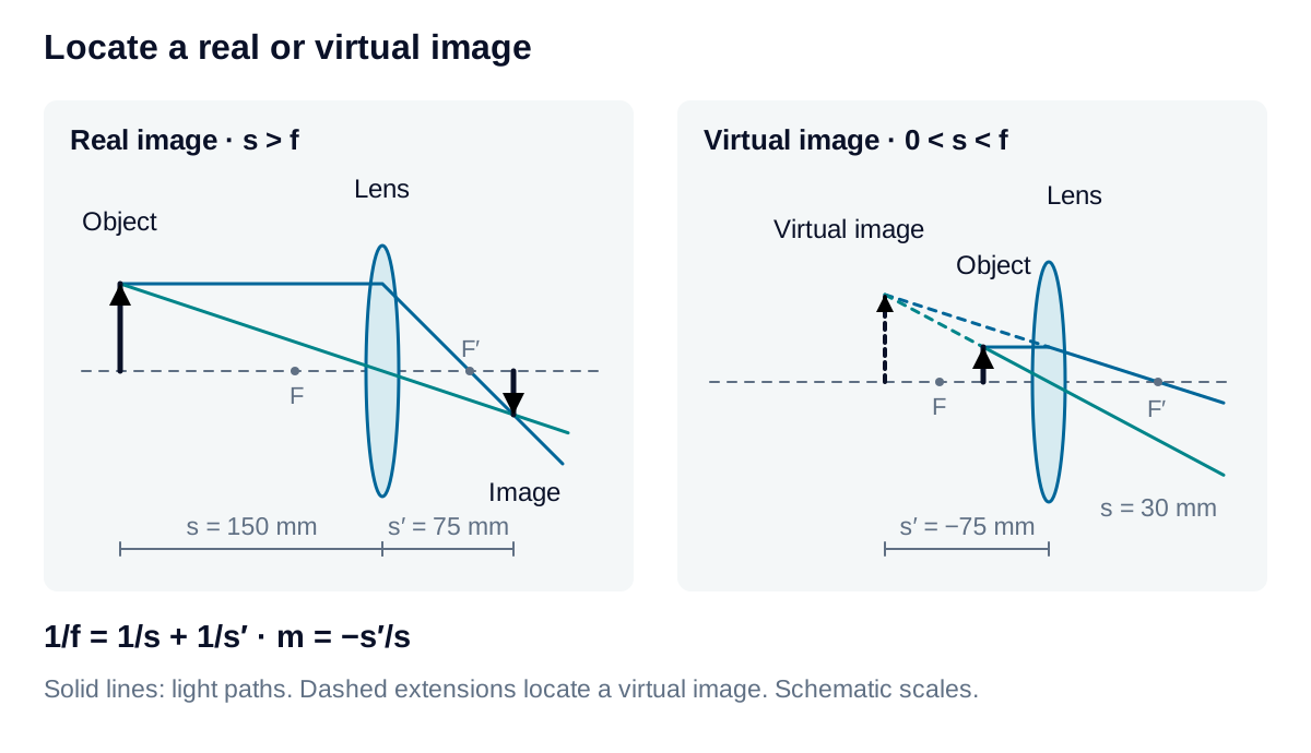
With mm and mm, the image lies 75 mm beyond the lens and . A 10 mm feature becomes a 5 mm inverted image. Moving a sensor to that image plane establishes geometric focus for the selected object plane.
Recognize the focal boundary
A converging lens has . Image distance grows as the object approaches the front focal plane from farther away. At , rays from each object point leave parallel, with no finite image plane or image height. Inside focus, the virtual image cannot be recorded by placing a bare sensor at its apparent location.
A diverging lens, , gives a real object a virtual, upright, reduced image. Following optics can still form another image.
Distinguish three magnification quantities
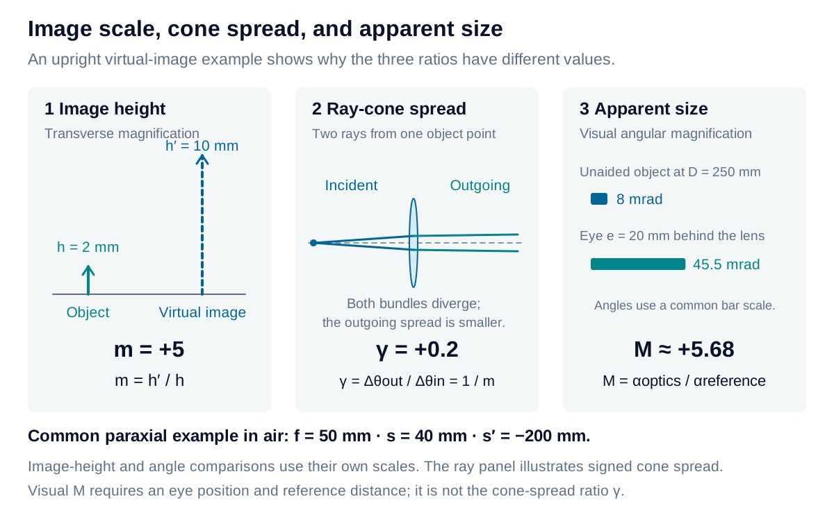
Image size, ray-cone spread, and apparent size describe different optical relationships. Use the quantity that matches the measurement, including its sign and reference conditions.
Transverse image magnification
The transverse magnification compares physical image height with object height:
Its magnitude gives the size ratio; its sign identifies orientation.
Derivation: transverse image magnification
In the thin-lens model with air on both sides, a ray through the lens center continues without changing direction. Place the object at axial position with height , and the lens center at position zero and height zero. The ray’s slope is:
At the image plane, axial position , the same line has height:
For a virtual image, extending the ray backward uses negative and gives an upright image for a real object. The relation describes a finite image; it does not assign a physical image height at infinity.
Signed cone-spread ratio
Consider two rays from the same object point. Let and be their signed paraxial angular separations, using one fixed transverse-axis convention. For finite conjugates in air, the ratio is:
The cone-width ratio is . A negative sign means a divergent bundle becomes convergent. At the focal condition, because the output is parallel; finite transverse magnification is then undefined.
Derivation: the cone-spread ratio is reciprocal to m
Use paraxial ray slope . Two rays from one object point reach the lens with height difference . Their incident slope difference is:
A thin lens changes each ray slope by . Subtracting the two ray equations and applying the lens equation gives:
Therefore, for a nonzero input spread and a finite image:
For example, corresponds to : an inverted image half as tall, with twice the angular cone width and opposite convergence sign. If , directly substituting into the slope difference gives zero output spread. No finite is assigned at that boundary.
This ratio concerns rays within one bundle. It does not compare the apparent angular size of an object with and without a viewing instrument.
Visual angular magnification
Visual magnification compares the angle an object subtends through the optics with its unaided angle at a stated reference distance . For an upright virtual image, , with the eye a distance behind the lens:
Unlike the cone-spread ratio, this result depends on the viewing geometry and comparison distance. A positive magnifier gives for a relaxed view at infinity; with the eye at the lens and the virtual image at distance , it gives .
Derivation: visual magnification and its viewing conditions
For object height and upright virtual-image height , the image lies a distance from the eye. In the small-angle approximation:
Taking their ratio yields . All lengths use the same units, and is measured from the unaided eye to the comparison object. The chosen rays must reach the eye without being clipped.
For relaxed viewing, place the object at the front focus of a positive lens. Its outgoing angle has magnitude approximately , so:
For a virtual image at the reference distance with the eye at the lens, and . Then:
The common choice mm is a comparison convention. It does not establish an individual’s near point or accommodation range. Moving the eye or changing the virtual-image location changes the general result.
Relate shape to power
For a thin lens of refractive index in air:
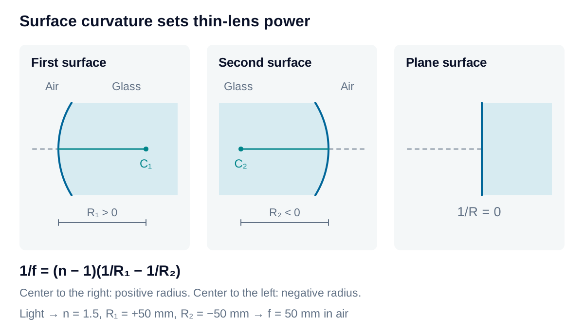
Light travels left to right; a radius is positive when its center of curvature lies to the right of that surface. A plane contributes zero curvature. For , mm and mm, the focal length is 50 mm. Use the material index at the operating wavelength.
Real assemblies introduce thickness, separated principal planes, aberrations, and aperture limits. Confirm the required field, working distance, and image quality with the lens specification before turning a first estimate into a measurement setup.