
Measurement System Analysis, or MSA, asks whether a measurement process supports its intended decision. Gage repeatability and reproducibility—Gage R&R—examines precision under a defined study design. It does not replace checks of bias, linearity, resolution, stability, calibration, or measurement uncertainty.
Separate the sources of variation
In a crossed study, each operator measures every part repeatedly. Equipment variation (EV) estimates repeatability within each part–operator combination. Appraiser variation (AV) describes operator differences. A part–operator interaction indicates that an operator’s effect depends on the part—for example, inconsistent alignment of particular surface geometries.
For an independent random-effects model:
Variances add; standard deviations do not. In the interaction model, the reproducibility component includes both operator and part–operator variation. Their relative sizes help distinguish a fixture or procedure problem from a broadly noisy measurement chain.
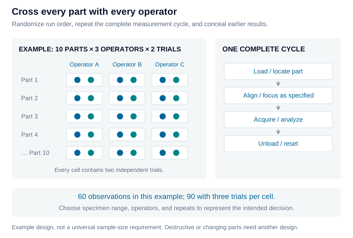
Build the study around actual use
A practical starting design is ten representative parts, three operators, and two or three trials per combination. This is an example, not a universal minimum. Parts should cover the relevant production range without being selected merely to inflate part-to-part variation. Operators, fixtures, environmental conditions, and repeated setup steps should represent the measurement process being qualified.
Randomize measurement order and conceal earlier results. For an optical station, repeating the complete load, align, focus, and measure cycle can reveal variation that repeated capture of an untouched sample cannot. Destructive tests or parts that change during measurement require a different design.
A practical crossed-study procedure
- Define the measurand, units, operating range, decision limits, and exact measurement procedure. Confirm calibration status, resolution, and a stable reference check before the study.
- Identify parts and operators independently of the measured value. Preserve specimen identity, condition, orientation, and any environmental or warm-up requirements.
- Have every operator measure every part in a randomized sequence. Repeat the full operational cycle for each trial; do not copy prior readings or reuse a fitted result as an independent measurement.
- Record part ID, operator ID, trial, result, time, and relevant conditions. Review missing cells, transcription errors, drift, outliers, and within-cell ranges before calculating components.
- Analyze the planned model. Inspect operator-by-part plots and residuals, including unequal spread or systematic drift; a single summary percentage cannot establish model validity.
- Compare measurement variation with the intended tolerance and actual process range. Investigate large components, improve the procedure or hardware, and repeat the study after a material change.
The calculator below provides a balanced crossed-study template. A part damaged during testing, a missing operator–part cell, or serial dependence cannot be repaired simply by averaging the available values.
Choose the analysis method deliberately
The average-and-range method uses repeated-measurement ranges and operator means to estimate components. It is transparent and useful for conventional balanced studies, but does not separately estimate part–operator interaction.
ANOVA fits part, operator, and interaction terms. A balanced crossed random-effects analysis separates these from residual repeatability. Model assumptions and interaction treatment must be reported; the selected parts and operators determine how far the conclusions generalize.
What ANOVA separates, and what ranges estimate
For part , operator , and trial , the crossed model is:
With parts, operators, and repeats, a balanced method-of-moments estimate uses ANOVA mean squares:
Finite data can produce negative component estimates. The calculator sets those estimates to zero for reporting and flags the boundary; zero is not proof that the underlying component is absent. It retains the interaction model rather than silently pooling an interaction into error.
For the average-and-range worksheet, let be the mean within-cell range, the range of operator grand means, and the range of part means. The standard-deviation estimates are:
The worksheet below supports ten parts, three operators, and two or three trials. It uses rounded constants for two trials or for three, , and . These are standard-deviation scale factors; the six-sigma study multiplier is applied afterward. Finite-sample corrections and tabulated constants differ between implementations, so report the actual convention rather than assuming all range methods are interchangeable. No separate interaction component is estimated in this worksheet.
The number of distinct categories, , estimates how well the measurement system distinguishes the sampled part variation. This worksheet convention reports:
This is a discrimination indicator, not an accuracy measure. With positive part variation and zero estimated Gage R&R, the ratio is unbounded; with both zero, it is undefined. Check resolution, rounding, and study size before interpreting either case as an exceptionally good instrument.
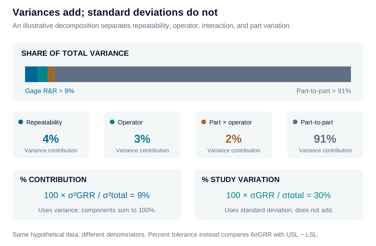
Read each percentage with its denominator
“Percent total” is ambiguous unless it identifies study variation or variance contribution. Mutually exclusive variance contributions sum to 100%; do not also add their R&R subtotal. Study variation depends on the sampled part range; tolerance percentage depends on engineering limits. Neither measures accuracy. Acceptance should reflect application risk and the agreed method, with uncertainty in the estimated components considered when the study is small.
Iris Optics can design and execute optical Gage R&R studies, identify dominant error sources, and improve fixtures, procedures, and analysis before production decisions depend on them.