
Two instruments can track the same changes and disagree on every result. Conversely, component and assembly measurements can be useful predictors without measuring the same quantity. Start a comparison by defining its purpose: establish agreement, characterize reproducibility, transfer a calibration, or predict performance.
Give the comparison a reference
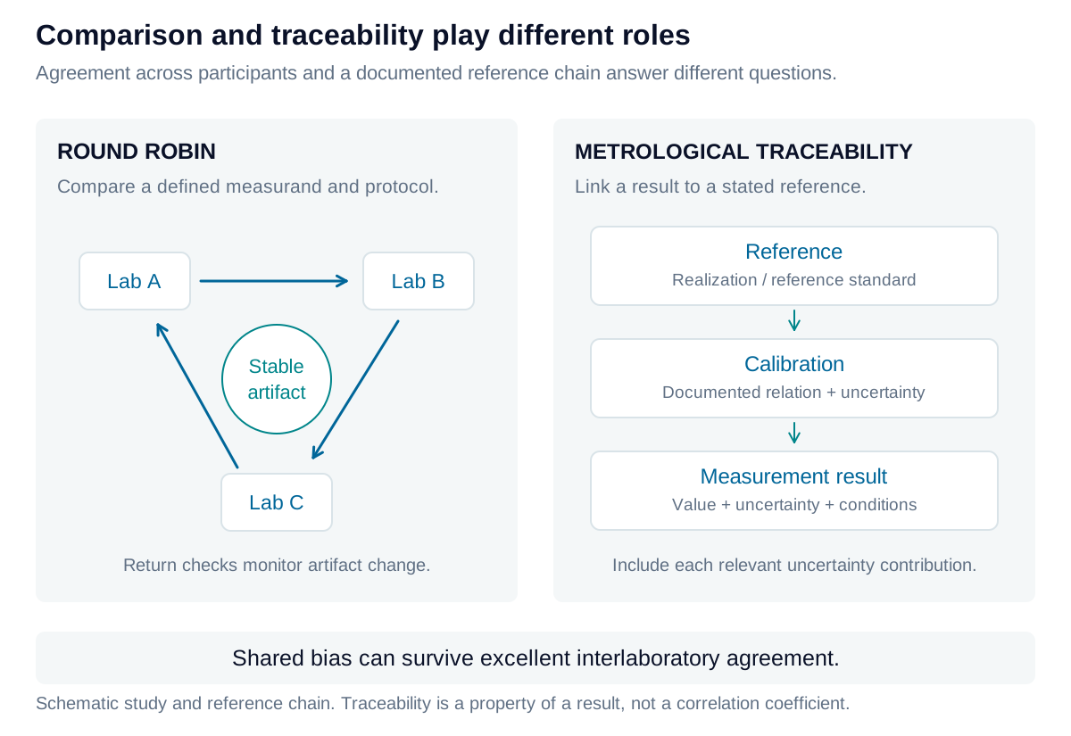
A round robin distributes stable specimens or reference artifacts among participants using a defined protocol. It can expose laboratory, instrument, fixture, and analysis differences before data are combined. Specify the measurand, units, geometry, environment, handling, repeated measurements, uncertainty reporting, and acceptance criteria. Monitor artifact stability during transport and use return measurements where practical.
Agreement among laboratories does not establish trueness: they can share a bias. Metrological traceability belongs to a measurement result linked to a reference through an unbroken, documented calibration chain, with uncertainty contributions. An instrument comparison or high correlation alone does not establish “NIST traceability.”
Separate agreement from association
For paired observations, Pearson correlation measures linear association:
It requires nonzero variation in both variables and is sensitive to outliers and range selection. A fitted straight line describes an intercept and slope . For ordinary least-squares regression with one predictor and an intercept, in-sample . This identity is not a general rule for arbitrary models or held-out prediction.
Spearman correlation applies Pearson’s calculation to ranks, with tied ranks averaged. It measures monotonic association and can detect a consistent curved relationship that a straight line summarizes poorly. Neither coefficient establishes agreement or causation.
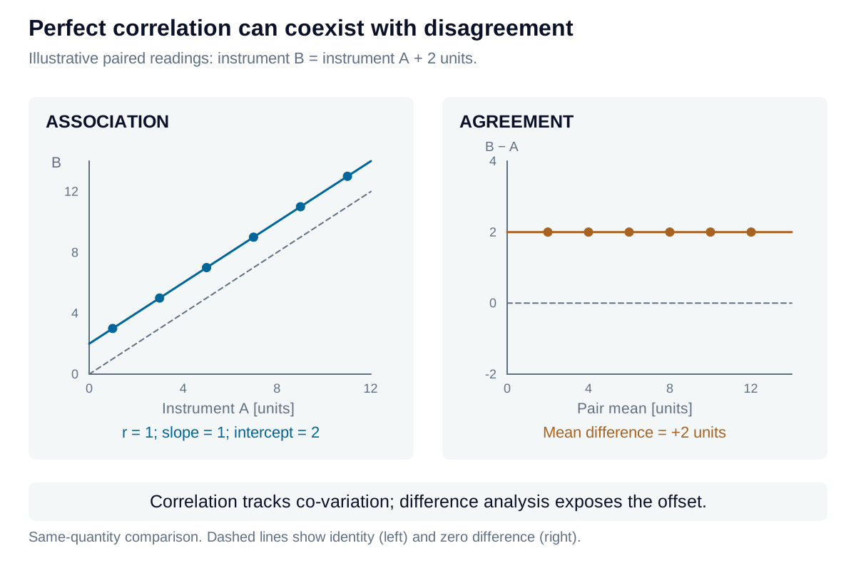
When both systems measure the same quantity, examine differences as well as a scatter plot. Plot against the pair mean. Mean difference estimates relative bias; approximately describes individual-difference limits when independent differences are suitably normal. These are not confidence intervals or engineering acceptance limits. Trends and changing spread require further modeling. If both axes have appreciable uncertainty, ordinary regression is generally inadequate for calibration transfer; an errors-in-variables method such as Deming regression requires an appropriate error-variance ratio.
Plan an instrument comparison or calibration transfer
Select paired specimens spanning the intended range and repeat measurements to characterize each system’s precision. Use the same measurand definition and compatible operating conditions; differences in wavelength, focus, ROI, filtering, or fit procedure can make nominally identical KPIs different quantities.
Plot paired values, the identity line, and pair differences. Check offsets, proportional effects, heteroscedasticity, outliers, and run-order drift. Where appropriate, estimate a transfer model using a reference with known uncertainty, then validate corrected results on independent specimens. Include transfer-model uncertainty and reference uncertainty in the result; a fitted slope is not a calibration certificate.
The calculator provides descriptive Pearson, Spearman, ordinary-regression, and same-quantity difference summaries. It does not perform Deming regression, an uncertainty budget, or a formal calibration.
Connect component measurements to system performance
Consider a hypothetical prism vendor reporting outgoing wavefront error while the assembled optical module is evaluated by MTF. These KPIs are related through optical performance but are not interchangeable. Match serialized components to assemblies and control wavelength, field, spatial frequency, orientation, focus, and alignment. Wavefront structure, not RMS magnitude alone, affects the resulting image. There is no universal conversion from one RMS wavefront number to assembly MTF.
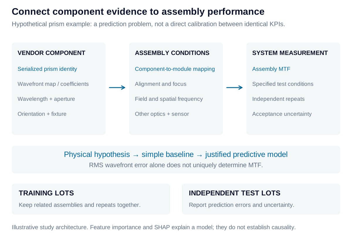
Begin with interpretable plots and a physical hypothesis. A nonlinear model may improve prediction, but it must outperform a simple baseline on independent production lots. Keep repeated measurements and related assemblies in the same data split to prevent leakage.
Where machine learning, mutual information, and SHAP help
Use multiple predictors when the engineering mechanism requires them: wavefront coefficients, surface form, orientation, assembly alignment, and test conditions may carry information lost in a single RMS value. Start with a simple regression and structured residual analysis. Compare a justified nonlinear method—such as a generalized additive model, kernel model, or tree ensemble—using held-out performance and prediction uncertainty.
Mutual information describes statistical dependence and can capture relationships that Pearson or Spearman correlation misses. It has no sign, its numerical scale is not a correlation coefficient, and its estimate depends on sample size and estimator settings. Feature screening must occur inside the training folds; small datasets can produce misleading apparent dependence.
SHAP attributes a fitted model’s predictions to its input features under a specified background distribution and attribution convention. It can help inspect whether a model relies on sensible predictors, but correlated inputs affect the attribution. SHAP values do not demonstrate a physical cause or validate the measurement itself.
For the prism example, reserve entire lots or later production periods for testing. Report prediction error at specified MTF conditions, inspect residuals by lot and field, and quantify uncertainty near acceptance boundaries. A strong relationship within one supplier’s existing process may not transfer after a material, alignment, or process change.
Iris Optics can establish comparable optical measurements across suppliers and laboratories, then develop validated component-to-system models that support practical engineering decisions.