
A calculated spectrum is the response of a particular model. A useful design must also satisfy the application across wavelength, angle, polarization, and expected manufacturing variation. Optimization connects these requirements to adjustable layer thicknesses, but an improved numerical score is only one part of the design decision.
Define the model before the objective
Specify the entrance medium, substrate, layer order, physical thicknesses, and wavelength-dependent refractive index and extinction coefficient. A coherent multilayer calculation combines fields and their phases; it cannot be replaced by adding interface reflectances. Power transmission also includes the ratio of exit to incident optical admittance.
Decide how the substrate’s rear surface is treated. A semi-infinite substrate omits it; a parallel finite substrate can introduce etalon fringes. Material dispersion, absorption, measurement bandwidth, and incidence geometry must represent the intended use. Bulk optical constants are a starting reference, not proof of a deposited film’s properties.
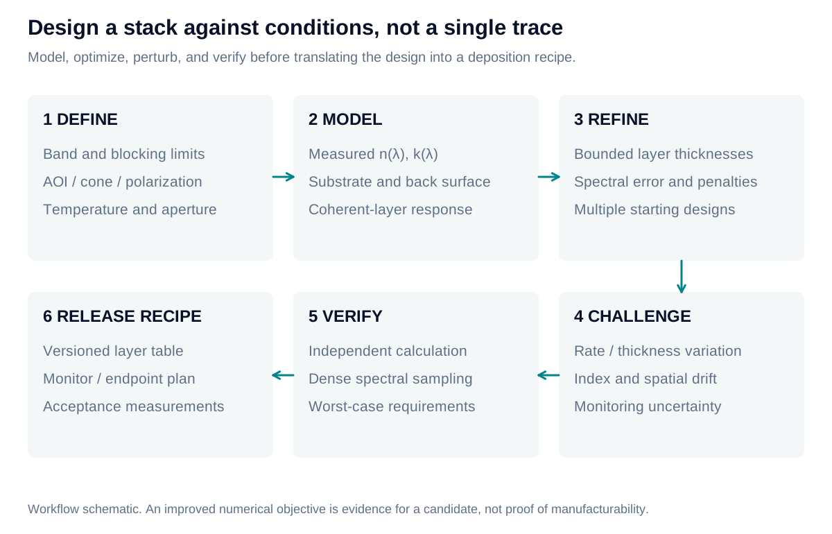
Choose a structure, then refine it
Begin with a physically appropriate seed: a matching stack for AR, a reflector for rejection, or coupled cavities for a shaped passband. Select which thicknesses may vary and apply bounds. A local optimizer can adjust this fixed structure efficiently, but its result depends on the starting point and allowed variables.
Structural changes address a different problem. Trial insertion of a thin layer can reveal an improving direction; subsequent refinement determines whether it remains useful. Added layers increase process burden, so remove or merge negligible layers only after recalculating the response. Convergence does not establish a global optimum or a manufacturable recipe.
Separate the score from compliance
For a target , let be its nonnegative violation and a positive normalization scale. An educational merit function is:
Here expresses relative priority. For an upper bound, ; reverse the difference for a lower bound. For an equality target, use . Compliance requires every entered target to be met. The normalization scale changes the score, not the acceptance limit; even can conceal failed requirements.
Choose weights, sampling, and acceptance rules deliberately
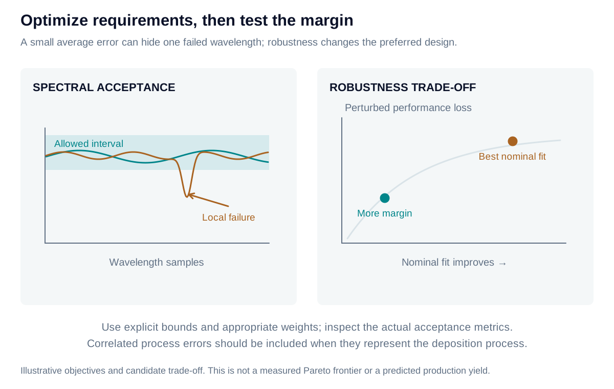
The calculator uses the displayed weighted RMS definition. Optimizers may instead minimize a worst residual, a goal-attainment parameter, or another objective. These formulations need not select the same design. Weighting changes the search preference; it does not relax a contractual acceptance limit.
For example, nine zero violations and one normalized violation of 2 produce an equally weighted score of approximately 0.63. The tenth requirement still fails. Likewise, acceptable transmission averaged across several angles does not prove that each angle passes. An unpolarized mean of s/p powers does not prove a requirement specified separately for both polarizations.
The calculator’s normalization scales do not add acceptance slack. For example, measured transmission of 94% fails a 95% minimum even with a scale of one percentage point. Numerical solver tolerance, contractual allowance, and physical manufacturing variation are distinct inputs. Preserve the best evaluated candidate and report bounds, solver status, objective, and individual requirement checks separately.
Test the sensitivity that remains
Recheck the candidate on a denser wavelength grid and across the complete angle and polarization range. Narrow leakage peaks can fall between optimization samples. Perturb thickness and optical constants using plausible independent and correlated process errors; a single perturbed example is not a yield estimate.
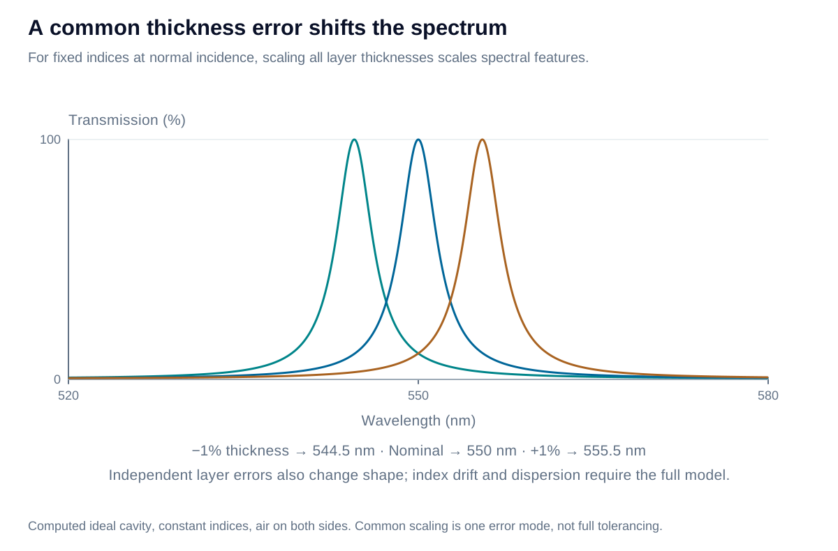
With fixed, nondispersive indices and fixed incidence, scaling every film thickness by scales corresponding spectral features by . Thus is a useful common-scale estimate. Individual-layer errors can also change ripple, width, and blocking; they cannot generally be represented by one wavelength shift.
Iris Optics can help define the optical model, acceptance criteria, and sensitivity study so that numerical refinement leads to a design that can be meaningfully manufactured and verified.