
A deposited filter must reproduce both its spectral response and its physical form. Thickness control matters, but so do optical constants, contamination, spatial uniformity, stress, and environmental stability. The coating design, deposition process, and acceptance metrology therefore need a shared definition of what constitutes a usable part.
Select the growth process
Evaporation and sputtering are physical vapor deposition methods. Sputtering uses energetic ions to release material from a target; DC, pulsed DC, AC, and RF are excitation choices suited to different targets and reactive processes. Chemical vapor deposition uses chemical reactions, while atomic layer deposition uses sequential, self-limiting surface reactions.
Process selection balances material compatibility, density, absorption, stress, uniformity, deposition rate, and substrate limits. Optical constants and layer rates should be characterized under representative process conditions rather than assumed from material names.
Observe growth in complementary ways
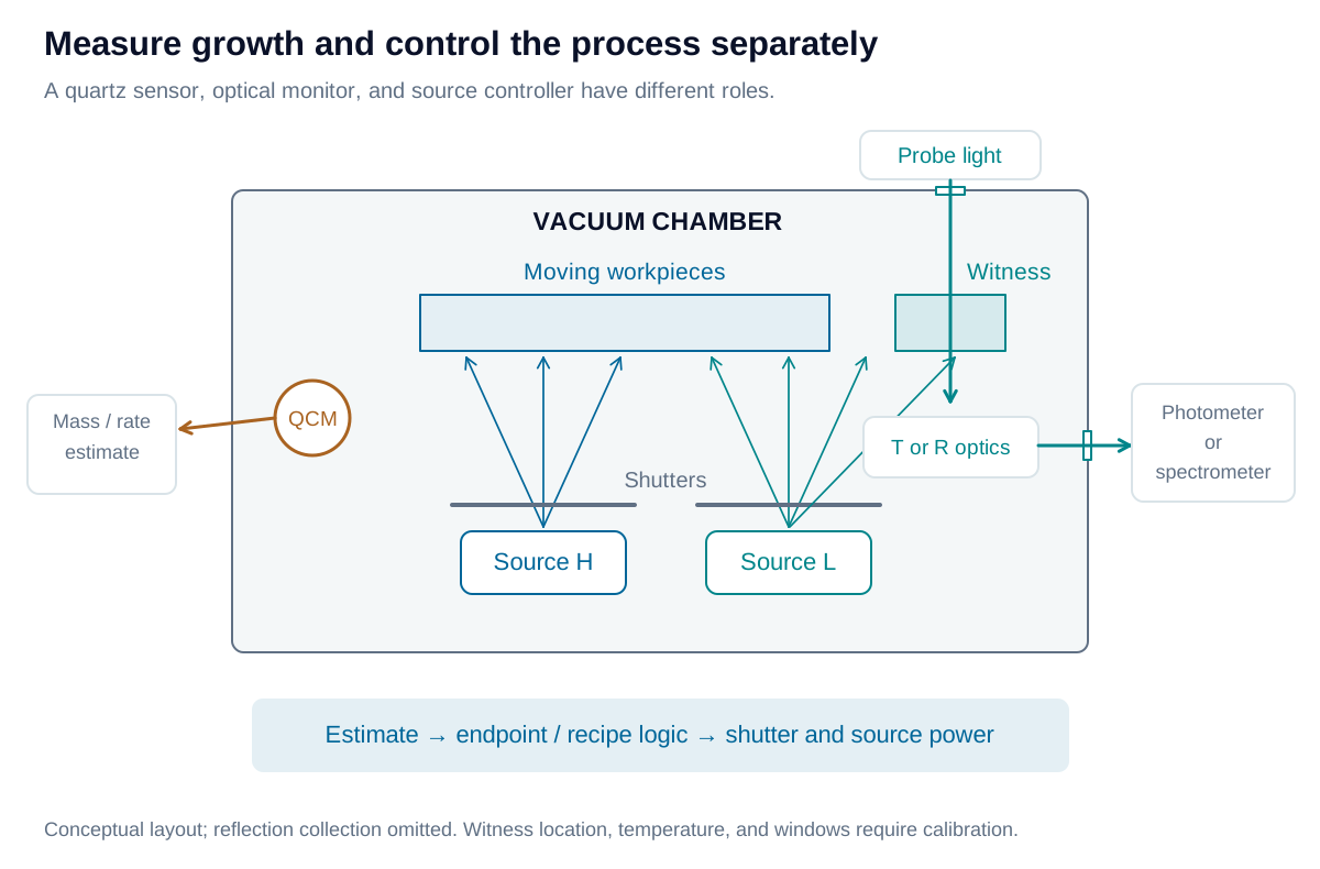
A quartz crystal monitor (QCM) infers deposited mass from a resonant-frequency change. Density and acoustic corrections convert that signal to thickness; a tooling calibration relates the crystal location to the workpiece. Rate feedback, including PID where appropriate, is a separate control choice.
An optical monitor measures evolving transmission or reflection through chamber windows, either on the workpiece or a representative witness. Single-wavelength measurements track a designed endpoint; broadband spectra provide more information for estimating thickness and diagnosing drift. Witness behavior must remain correlated with the coated parts.
Terminate layers and manage drift
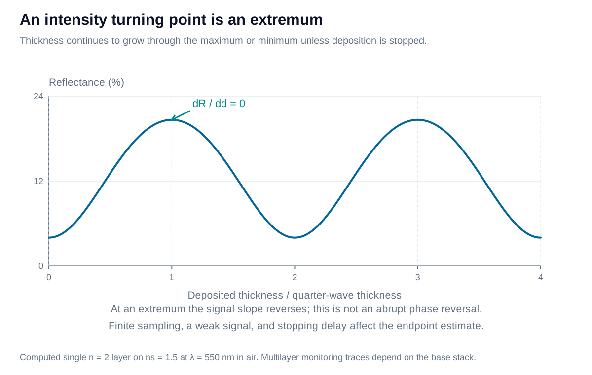
A turning point is an intensity maximum or minimum where the monitoring trace reverses slope. Quarter-wave and multiple-quarter-wave structures can provide convenient extrema at a selected wavelength. This is not a sudden phase jump, and arbitrary layer designs require other endpoint strategies.
At approximately constant rate , an effective stopping delay adds:
The second expression is the one-way phase-thickness error at normal incidence. A predictable delay can be compensated in the endpoint strategy; rate drift and noise still require evaluation.
Understand what a turning point can reveal
As a transparent layer grows, the returning field rotates in phase and the detected intensity rises or falls. In an ideal quarter-wave monitoring sequence, the chosen endpoint coincides with an extremum. Near that extremum the first derivative of intensity with thickness is zero, so a single noisy intensity sample has limited thickness sensitivity. Trace fitting, sampling cadence, calibrated delays, and the response of the layers already deposited affect the endpoint estimate.
An arbitrary non-QW layer may end away from an extremum. Its monitor wavelength, signal target, broadband fit, or combined optical/QCM strategy must be designed accordingly. The same growing layer can produce different traces at different wavelengths. The plot illustrates the interference mechanism rather than a universal coater waveform.
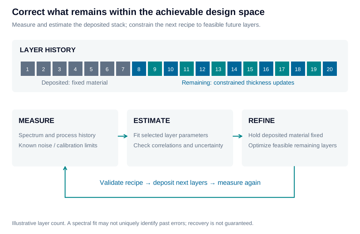
Measured spectra can also support remaining-layer reoptimization: estimate the deposited structure, hold it fixed, and adjust future layers within feasible bounds. This may recover an acceptable response, but cannot remove material already deposited. Several thickness-error combinations can explain similar spectra, so uncertainty and model ambiguity limit the correction.
Choose a recovery cadence and preserve feasible corrections
For a 200-layer design, a checkpoint after layer 10 leaves 190 layers available for correction; after layer 20, 180 remain. The useful measurement cadence depends on observability, cycle time, and spectral sensitivity rather than a universal interval.
A recovery loop compares measured and predicted spectra, estimates only supported process parameters, and propagates their uncertainty. It then refines the remaining layer thicknesses, checks the predicted response and manufacturing bounds, and releases a revised continuation recipe. Independent material information or accumulated monitoring history can help distinguish index drift from thickness error. A witness that does not represent the workpiece can lead the correction in the wrong direction.
Preserve form and verify usable parts
Coating stress can bend the substrate and introduce surface form error (SFE). A backside stress-balancing AR coating can reduce that bending while controlling rear-surface reflection. Balance depends on stress times thickness, not equal coating thickness alone. Improved flatness does not automatically improve transmitted wavefront error: coating nonuniformity and optical phase also contribute.
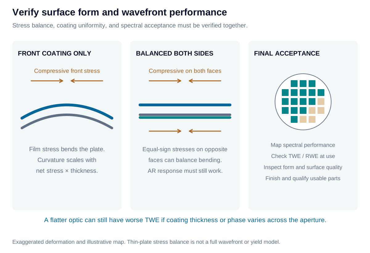
Map spectral performance over the clear aperture using the specified wavelength resolution, angle, and polarization. Verify surface quality, form, wavefront, and required durability. Measure transmitted or reflected wavefront at the use wavelength and angle, or apply a validated conversion from the test conditions. Wafer-based production can use these maps before singulation, followed by final inspection; individually coated optics follow their own acceptance route.
Estimate bow from stress-thickness balance
For a thin uniform coating on an isotropic elastic substrate, define signed stress-thickness in N/m, with tensile stress positive on either face. Let and denote the front and back totals. The thin-film Stoney approximation gives the change in curvature:
Here is substrate thickness and its biaxial modulus. Equal signed stress-thickness on opposite faces cancels ideal bending; opposite signs can reinforce it. For an initially flat, free plate and small slopes, the center-to-rim sag magnitude across diameter is approximately .
This estimate assumes coatings much thinner than the substrate, uniform equibiaxial stress, and negligible film bending stiffness. It does not predict adhesion, fracture, mounted deformation, or optical wavefront error. Spatially varying coatings and anisotropic substrates require a more complete model.
Iris Optics can develop monitoring and acceptance methods that connect spectral performance, surface form, and measurement capability, helping teams distinguish process drift from measurement artifacts and identify usable parts.