01 / 03 Sensor principles

Application note

Selecting Optical Distance and Displacement Sensors

Match the ranging principle, surface response, and spatial coverage to the measurement task.

Try the application calculators ↓ Discuss your application →

An optical distance sensor infers surface position from light received through a particular geometry. Displacement is the change between positions. A small displayed increment does not establish equally small measurement uncertainty: surface finish, tilt, motion, temperature, and the reference frame all affect the result.

Choose what to measure, then how much to capture

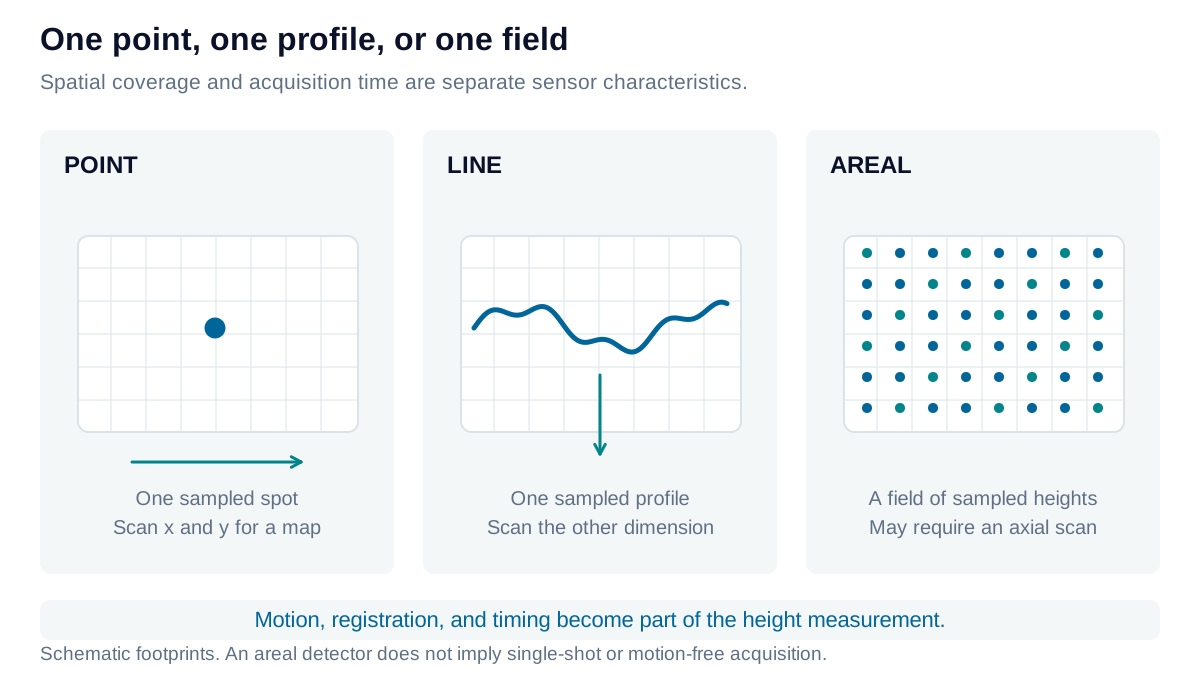
A point sensor samples a spot; a line sensor samples a profile; an areal system samples a field. Motion can assemble points or profiles into a surface map, but encoder errors, vibration, and synchronization then become part of the measurement. An areal instrument may also require multiple exposures or an axial scan.

Point, line, and areal acquisition sample different spatial footprints. Scanning adds another coordinate and its positioning errors.

View diagram at full size

Encode depth as position, focus, or wavelength

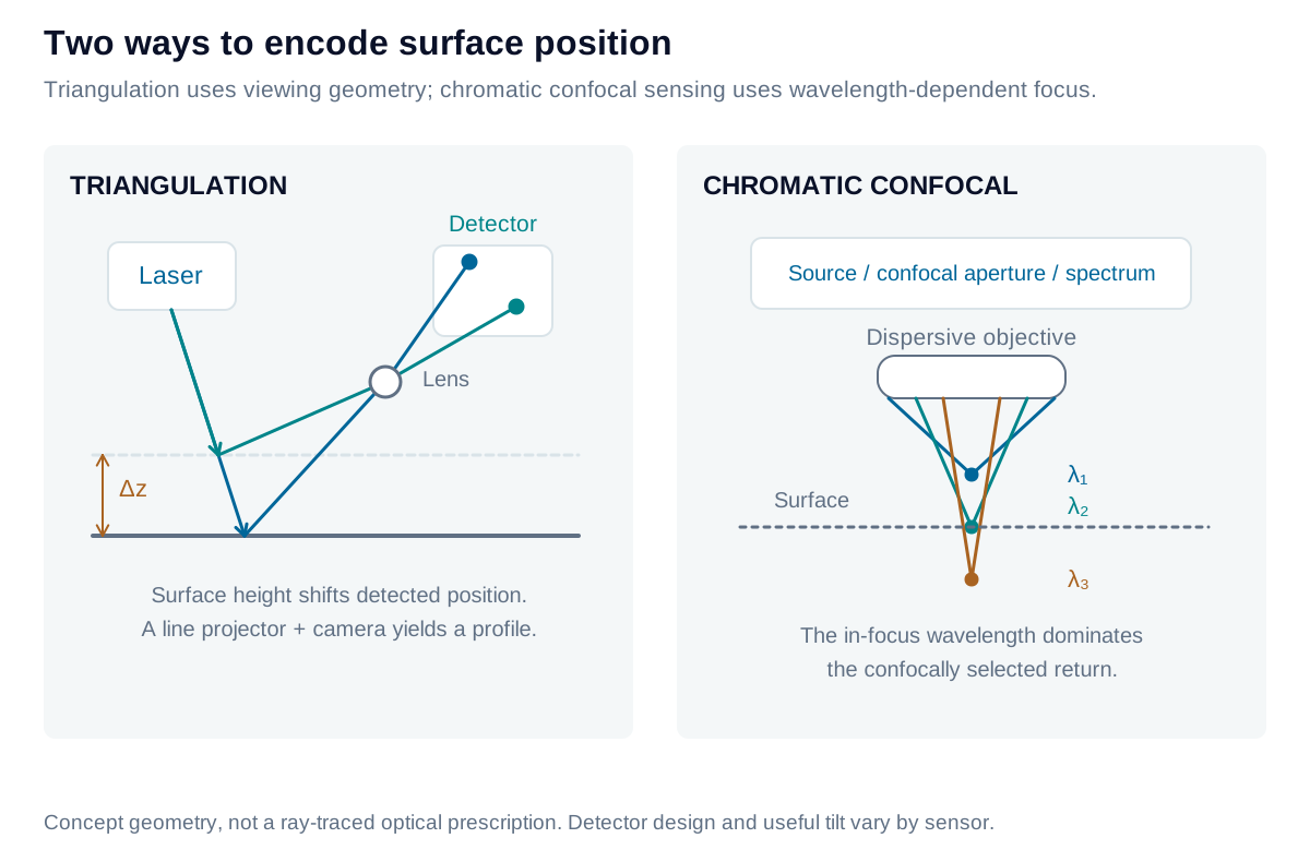
Laser triangulation observes an illuminated spot from an offset receiving aperture. Height changes shift the spot on a position-sensitive detector or camera. A projected line and two-dimensional camera extend this geometry to a profile. Detector format varies by implementation. Diffuse and specular configurations require different receiving geometries; a specular surface can lose signal abruptly when tilted.

Scanning confocal locates the axial intensity maximum as the focus moves. Chromatic confocal deliberately separates focal positions by wavelength; a calibrated spectral peak identifies depth without mechanically sweeping the focus. High numerical aperture can collect returns from steeper surfaces, with working-distance and spot-size tradeoffs. Line confocal systems extend spatial coverage using specialized optical encoding; their architectures are not all equivalent to adding a detector dimension.

Triangulation changes detected position with height; chromatic confocal ranging maps the wavelength that focuses on the surface to axial position.

View diagram at full size

Encode optical path through interference

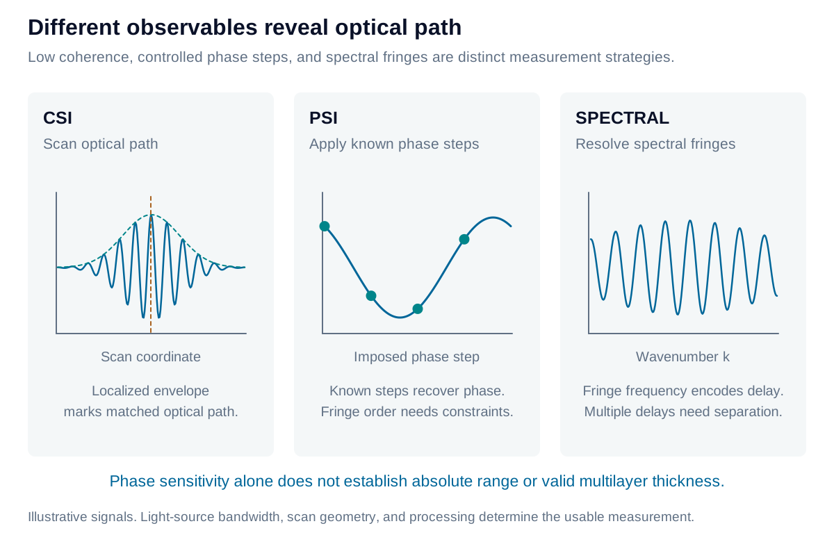
Coherence scanning interferometry (CSI) scans optical path through a localized fringe envelope using a low-coherence source. Phase-shifting interferometry (PSI) introduces known phase steps and solves fringe phase, requiring phase unwrapping or other constraints when the surface spans ambiguous orders. Spectral interferometry measures interference against wavelength or wavenumber to recover optical delays; a swept source is a frequency-domain implementation, rather than a mechanical CSI scan.

These methods may use point or areal detection. Their angular acceptance depends on the actual aperture, reference geometry, and surface scattering—not on “interferometry” as a single category.

For a single reflected beam, an unwrapped phase change $\Delta\phi$ gives normal displacement:

\Delta z=\frac{\lambda_0\Delta\phi}{4\pi n\cos\theta}

Here $\lambda_0$ is vacuum wavelength, $n$ is the propagation-medium phase index, and $\theta$ is incidence from the surface normal. Positive phase denotes increasing optical path; phase alone does not establish absolute range.

CSI finds a localized fringe envelope, PSI measures phase changes, and spectral interferometry recovers optical delay from spectral fringe frequency.

View diagram at full size

Distinguish height coding from slope sensing

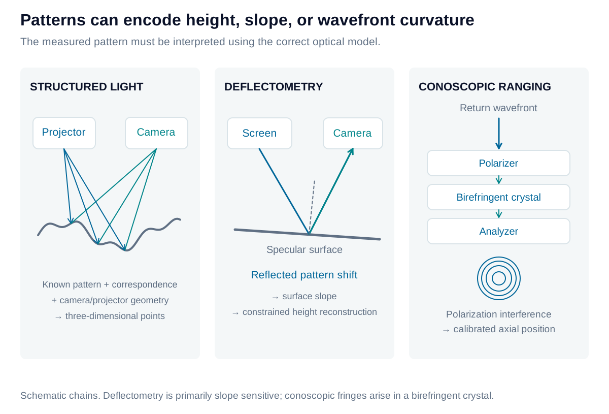
Structured light projects identifiable patterns and triangulates corresponding camera observations into three-dimensional points. Deflectometry observes a known pattern reflected by a specular surface. Pattern displacement primarily encodes surface slope; recovering height requires calibrated geometry and a reconstruction constraint.

Conoscopic holography sends returned light through polarization optics and a birefringent crystal. Two polarization components acquire different angle-dependent phases and interfere after an analyzer. The resulting fringe pattern encodes wavefront curvature, which a calibrated model converts to axial distance. It uses a nearly common optical path rather than a conventional separated reference arm.

Structured light triangulates projected features; deflectometry measures reflected-pattern deflection; conoscopic ranging decodes polarization interference.

View diagram at full size

How a conoscopic fringe pattern encodes distance

Light returning from a small illuminated surface region forms a wavefront whose curvature depends on the region’s axial position and the receiving optics. In a uniaxial birefringent crystal, the ordinary and extraordinary polarization components propagate with different effective refractive indices. Their phase difference depends on propagation direction through the crystal.

An analyzer combines both components into a common polarization so that they can interfere. The detector records a spatial fringe pattern, often represented as rings in a symmetric configuration. Changing object position changes the wavefront presented to the crystal and therefore the measured fringe scale or spatial frequency. The instrument converts that pattern to distance using its calibrated optical geometry.

The two components largely share the same path, which reduces some differential-path disturbances. It does not eliminate surface-dependent errors, vibration, fringe ambiguity, or the need to calibrate the instrument’s operating interval. The measurement is a position estimate from a fringe pattern, rather than a reconstructed photographic hologram of the object.

Additional methods and practical limits

Pulsed time of flight measures round-trip delay, with $z=c\Delta t/(2n_g)$ in a uniform medium. Continuous-wave phase ranging instead measures modulation phase and has an ambiguity interval. FMCW LiDAR mixes a frequency-chirped return with a reference; beat frequency estimates delay, while target velocity can contribute a Doppler term. These methods suit longer ranges, subject to bandwidth, signal level, multipath, and motion constraints.

Laser Doppler vibrometry measures the Doppler shift of returned light, principally providing velocity along the sensitivity direction. Displacement can be obtained by integration or appropriate demodulation, but drift and reference conditions matter. It is not automatically an absolute stand-off measurement.

Focus variation estimates height from the focus position that maximizes local image sharpness. It benefits from surface texture; smooth transparent or mirror-like regions may supply too little usable contrast. A visually sharp focus-stacked image is not, by itself, a calibrated height map.

For a simple single-sided acceptance cone in air, $NA=\sin\alpha$ . This optical collection angle is not a universal allowable surface slope. Specular reflection changes return direction by approximately twice the surface tilt, while illumination and collection pupils may overlap differently in each architecture. Confirm usable tilt on representative material rather than converting NA directly into a guaranteed sensor specification.

Compare the complete measurement chain

Keep stand-off, axial measurement range, lateral sampling, resolution, repeatability, and linearity separate. Specify the averaging, bandwidth, target, and environment behind each number. The comparison below is a screening aid; a weighted preference cannot compensate for a failed material, access, speed, or uncertainty requirement.

Iris Optics can evaluate representative parts, compare viable sensing principles, and develop the fixture, motion, calibration, and analysis needed to turn a sensor specification into a dependable measurement system.

From principle to selection

Build a sensor selection matrix

Use a Kepner–Tregoe-style decision sequence: define mandatory requirements first, then score the preferences that distinguish feasible options. Surface compatibility, clearance, usable range, uncertainty, and required production speed are useful first gates. A missing specification requires a test or quotation.

For the remaining options, assign weights to the criteria and scores against the same evidence: S = Σ wᵢsᵢ. A high weighted score cannot rescue a failed mandatory requirement. Review implementation risks before selecting a system.

Range and vertical sensitivity span different scales

These named examples give the trade-off map a numerical scale. They are individual configurations, not technology-wide limits. Circle markers report repeatability; diamonds report a manufacturer's resolution or dynamic-noise value. Averaging and test conditions differ, so proximity on this plot does not establish equivalent performance.

Blue: point triangulation. Amber: line triangulation. Teal: chromatic confocal. ● Repeatability. ◆ Resolution/noise specification. The two IFS2405 examples use the same 1 kHz dynamic-RMS definition: a longer-range probe also has a larger quoted noise bound. Other comparisons require matched tests.

Read the six plotted specifications and their conditions

1. KEYENCE LK-H020

6 mm axial span; 20 mm reference distance; nominal interval 17–23 mm. repeatability: 0.02 µm (published value).

Standard target at reference distance; 16,384-reading averaging. Not single-shot or maximum-rate precision.
25 µm spot; linearity ±0.02% of 6 mm full scale under the specified reference-target conditions.
2. KEYENCE LJ-X8020

4.4 mm axial span; 20 mm reference distance; nominal Z interval 17.8–22.2 mm. repeatability: 0.3 µm (Z-height, averaged region).

Standard target at reference distance; 4,096-reading averaging; average height of the default region. Not per-pixel single-shot noise.
7.5 mm profile width at reference; 2.5 µm nominal X interval. Maximum 16 kHz requires restricted range/binning conditions.
3. Micro-Epsilon ILD2300-2

2 mm axial span; 24 mm start of measuring range; nominal interval 24–26 mm. resolution: 0.03 µm (manufacturer resolution).

20 kHz measuring rate; white diffuse reference ceramic. This resolution is not the repeatability metric used by other rows.
Linearity < ±0.6 µm; approximately 23 × 23 µm spot at midrange. Electronics are integrated.
4. Micro-Epsilon IFS2405-0.3

0.3 mm axial span; 6 mm approximate start of measuring range; interval about 6–6.3 mm. resolution: < 0.018 µm (dynamic RMS-noise upper bound).

Dynamic resolution <18 nm at midrange, 1 kHz. Separately, static <2 nm uses 512-reading averaging; do not combine these conditions.
6 µm spot; NA 0.60; usable mirrored-surface signal to ±34°, with accuracy degrading near the angular limit.
5. Micro-Epsilon IFS2405-6

6 mm axial span; 63 mm approximate start of measuring range; interval about 63–69 mm. resolution: < 0.19 µm (dynamic RMS-noise upper bound).

Dynamic resolution <190 nm at midrange, 1 kHz. Static <17 nm uses averaging. Compare configurations using the same metric and bandwidth.
31 µm spot; NA 0.22; usable mirrored-surface signal to ±10°, with accuracy degrading near the angular limit.
6. LMI FocalSpec LCI1220

3 mm axial span; 20.6 mm manufacturer stand-off specification. repeatability: 0.19 µm (published Z repeatability).

Manufacturer summary does not fully state the repeatability protocol. 3,000 profiles/s at full range; 16,000 profiles/s is a separate maximum.
11.6 mm field; 6.7 µm X sampling; stated mirror-surface slope limit ±20°. Off-axis line-confocal architecture.

Technology selection matrix

The same thirteen technology families appear in each part of the matrix. Use these prompts to define the test conditions and the evidence required from a supplier. The named specifications above illustrate selected configurations; a family does not have one universal numerical range, spot size, or repeatability.

Compare range, stand-off, and axial performance

Compare range, stand-off, and axial performance
Technology	Measurement range	Stand-off / clearance	Resolution	Repeatability / precision	Linearity
Point laser triangulationKEYENCE LK-G5000; Micro-Epsilon optoNCDT ILD2300	Head-specific axial span; more span usually trades away height sensitivity.	Separate reference distance from the usable near-to-far interval.	Image localization and signal quality limit usable changes; display digits are insufficient.	Target finish, speckle, averaging, and bandwidth matter.	Check the calibrated depth interval and the stated target material.
Laser line triangulationKEYENCE LJ-X8000; Micro-Epsilon scanCONTROL	Specify both Z span and X field width; width can vary with depth.	Reference distance fixes clearance and the near/far profile widths.	X sample pitch, laser width, and Z discrimination are different specifications.	Averaged area height can be much more stable than individual profile points.	Check smoothing and averaging used for the published value.
Coherence scanning interferometryZygo NewView 9000; KEYENCE WI-5000; Bristol optical thickness gauges	Scan travel, objective clearance, surface slope, and usable signal constrain the height span.	Objective- or probe-dependent; long stand-off is not intrinsic to CSI.	Nanometer-scale height sensitivity can coexist with micrometer-scale lateral detail.	Specify scan mode, averaging, vibration, surface, and the reported height statistic.	Vertical amplification, scan mechanics, and material phase response need calibration.
Phase-shifting interferometryTRIOPTICS µPhase; Zygo SmartPSI modes	Phase is modulo 2π; discontinuities require unwrapping or an additional ranging method.	Set by the interferometer, reference optics, and test geometry.	Small phase changes give high height sensitivity; not absolute-distance range.	Report a surface/wavefront statistic and aperture, not just a nominal phase increment.	Phase-step error, reference quality, retrace, and calibration affect the result.
Spectral interferometryKEYENCE SI-F series; PRECITEC CHRocodile interferometric sensors	Spectral span, spectral sampling, and probe geometry bound resolvable delays.	Probe-specific; distinguish target detection distance from thickness/gap range.	Delay separation and peak-position precision are different limits.	Keep averaging, bandwidth, return strength, and material dispersion attached to the value.	Wavelength/frequency calibration and the material model enter the distance scale.
Axially scanning confocalKEYENCE LT-9000 documented scanning-confocal architecture	Focus travel and the calibrated optical scan establish the usable depth span.	Objective- or head-specific clearance.	Focus-peak localization depends on NA, signal, and the Z sampling strategy.	Scan mechanics, reflected signal, and target texture affect repeat measurements.	Verify the Z drive or internal scan calibration.
Chromatic confocalMicro-Epsilon confocalDT; KEYENCE CL-3000; PRECITEC CHRocodile; LMI FocalSpec	Probe-specific chromatic focal span; increasing span often reduces axial sensitivity.	Probe-specific; inspect the near limit, not only nominal working distance.	Static averaged resolution can differ greatly from dynamic RMS noise.	Spectral signal, reflectance, rate, and peak processing affect the result.	Probe/controller calibration and the refractive-index model matter for thickness.
Structured-light triangulationTI DLP structured-light reference architectures; Micro-Epsilon surfaceCONTROL	Calibrated measurement volume; scaling the volume trades against spatial detail.	Projector/camera baseline, optics, and desired coverage determine clearance.	Depth sensitivity and lateral sample spacing are separate.	Exposure sequence, pattern contrast, calibration, and surface response matter.	Validate volumetric geometry with traceable artifacts across the working volume.
DeflectometryMicro-Epsilon reflectCONTROL	Slope range and geometric coverage are more meaningful than a universal axial span.	Screen, camera, and sample geometry jointly determine the working volume.	Slope sensitivity must not be relabeled as height resolution.	Pattern phase, calibration, and height reconstruction affect repeat results.	Validate reconstructed shape and relevant spatial scales.
Conoscopic holographyOptimet ConoProbe / ConoPoint documented examples	Objective-specific; changing optics changes depth span and sensitivity.	Objective-specific; coaxial access can help with narrow features.	Fringe estimation and calibration determine axial discrimination.	Return power, surface geometry, and signal processing must be specified.	Calibrate the fringe-pattern-to-distance relationship over the selected objective range.
Time of flight / FMCW rangingMicro-Epsilon optoNCDT ILR; ST FlightSense ToF; Aeva FMCW LiDAR	Often selected for larger distances; choose a specific instrument and target return.	Minimum usable range and maximum return-limited range both matter.	Timing or sweep bandwidth sets range discrimination; fitted range precision is a separate metric.	Reflectance, ambient light, multipath, integration time, and motion matter.	Timing/sweep calibration and range-dependent bias need verification.
Laser Doppler vibrometryPolytec vibrometers	Specify vibration amplitude and frequency bandwidth, not a static thickness span.	Focus, return level, and model determine working distance.	Displacement noise depends on frequency bandwidth and demodulation.	Dynamic signal, speckle dropouts, alignment, and bandwidth matter.	Velocity/displacement decoder calibration is relevant.
Focus variationBruker Alicona focus-variation systems	Z travel, optical focus, and surface texture bound the reconstruction.	Objective-dependent clearance.	Lateral texture, depth of field, Z scan, and focus estimator all contribute.	Texture contrast and the scan/reconstruction settings must be held fixed.	Verify the calibrated Z scale and reconstruction against suitable artifacts.

Compare slope acceptance, sampling, and integration

Compare slope acceptance, sampling, and integration
Technology	Point, line, or area	Angular acceptance	Sampling / map rate	Spot / lateral sampling	Inline or benchtop
Point laser triangulationKEYENCE LK-G5000; Micro-Epsilon optoNCDT ILD2300	Point; scan motion adds profiles or maps.	Diffuse and specular layouts differ; shadowing and the return direction limit access.	Fast single-point acquisition; filtering reduces effective response.	Focused spot or short averaging line; the latter is not a measured profile.	Inline heads; some integrate electronics, others need a controller.
Laser line triangulationKEYENCE LJ-X8000; Micro-Epsilon scanCONTROL	Line; an encoder and perpendicular motion build an areal map.	Receiver baseline creates shadows; mirror returns need a suitable orientation.	Profile rate changes with ROI, binning, exposure, and processing.	A finite-width illuminated line, not independent ideal point probes.	Inline profiling; motion and encoder errors enter the areal result.
Coherence scanning interferometryZygo NewView 9000; KEYENCE WI-5000; Bristol optical thickness gauges	Point or areal, depending on instrument architecture.	High-NA objectives can accept steep slopes; field width and working distance may shrink.	Areal scan time is not a per-pixel sampling frequency.	A point probe or an objective-defined lateral response across an image.	Benchtop and OEM/production systems; vibration control remains application-specific.
Phase-shifting interferometryTRIOPTICS µPhase; Zygo SmartPSI modes	Commonly areal surface or wavefront testing; point implementations also exist.	Depends on objective/test-wave geometry and fringe sampling; not universally low NA.	Multiple phase frames or simultaneous phase channels; motion during capture matters.	Imaging aperture and lateral optical response, rather than one universal spot size.	Laboratory, production, and embedded implementations with appropriate stability.
Spectral interferometryKEYENCE SI-F series; PRECITEC CHRocodile interferometric sensors	Point probes; scanning or parallel acquisition can add coverage.	Return collection and spot geometry dominate; a narrow probe can require careful alignment.	Spectrometer acquisition or wavelength sweep rate; reported output may be averaged.	Probe focus and depth of field determine the illuminated region.	Inline point systems and laboratory instruments.
Axially scanning confocalKEYENCE LT-9000 documented scanning-confocal architecture	Point, scanned line, or areal microscope implementations.	Illumination/collection aperture and surface scattering determine accepted slopes.	A complete focus scan is needed; do not substitute camera rate for height-map rate.	Objective-dependent focused spot; remains near focus as the scan proceeds.	Inline scanning heads and laboratory scanning microscopes.
Chromatic confocalMicro-Epsilon confocalDT; KEYENCE CL-3000; PRECITEC CHRocodile; LMI FocalSpec	Point, multipoint, and line; line designs use additional spatial encoding.	High NA can improve slope acceptance, with a working-distance/range trade-off.	Spectral acquisition and available return light limit point or profile rate.	Small point spots or a line of finite lateral samples; check both lateral axes.	Widely used inline; passive probe heads may connect to separate spectral electronics.
Structured-light triangulationTI DLP structured-light reference architectures; Micro-Epsilon surfaceCONTROL	Areal; multiple pattern exposures are common.	Both projector and camera must see the surface; deep cavities cause occlusion.	Pattern rate is not complete 3D-map rate; motion can break correspondence.	Projected pixels and imaged surface detail replace a single beam diameter.	Inline, robot-mounted, and benchtop systems; geometry calibration is central.
DeflectometryMicro-Epsilon reflectCONTROL	Areal; height reconstruction requires additional geometry and constraints.	A valid reflected path must connect screen, surface, and camera.	Pattern sequence, exposure, and reconstruction set the map rate.	Camera sampling and reconstruction bandwidth define lateral detail.	Inline inspection and benchtop form/defect systems.
Conoscopic holographyOptimet ConoProbe / ConoPoint documented examples	Point probes; scanning builds profiles/maps; line architectures have been demonstrated.	Coaxial access reduces triangulation shadowing; published steep-angle claims depend on surface scattering.	Sensor- and signal-dependent; inspect the actual acquisition configuration.	Objective-dependent illuminated spot; not the fringe diameter on the detector.	Documented inline and CMM-integrated probes; confirm current supply and support.
Time of flight / FMCW rangingMicro-Epsilon optoNCDT ILR; ST FlightSense ToF; Aeva FMCW LiDAR	Point, scanned, or array sensors.	Return strength and footprint vary with incidence; no universal slope limit.	Distinguish individual returns, point-cloud rate, and full-frame rate.	Beam divergence or pixel field of view grows the footprint with distance.	Inline positioning, robotics, and larger-volume ranging.
Laser Doppler vibrometryPolytec vibrometers	Point; scanning maps vibration over selected locations.	Measures the velocity component along the beam; surface return must be sufficient.	Frequency bandwidth and sampling rate need separate specifications.	Focused measurement spot; scanning location is not continuous areal capture.	Laboratory and industrial end-of-line vibration testing.
Focus variationBruker Alicona focus-variation systems	Areal, often with stitched fields.	Textured steep surfaces can be accessible if illumination and viewing remain adequate.	Full Z-stack acquisition and reconstruction determine map time.	Image neighborhood used by the focus measure; not a point beam.	Benchtop and automated metrology systems.

Compare head, controller, and complete-system cost

The reviewed suppliers do not provide a verified public price for a comparable installed configuration. Request head, controller, optics, software, motion, fixture, and calibration costs separately; a used head or development-board price is not a system budget.

Configured system cost requirements
Technology	Sensor head	Controller / electronics	Complete system	Budget boundary
Point laser triangulation	Request a configured quote	Integrated on some heads; external on others	No verified public installed-system price	Budget the complete configuration, fixtures, motion, calibration, software, and integration.
Laser line triangulation	Request a configured quote	Confirm required electronics and licenses	No verified public installed-system price	Budget the complete configuration, fixtures, motion, calibration, software, and integration.
Coherence scanning interferometry	Request a configured quote	Usually part of a configured instrument	No verified public installed-system price	Budget the complete configuration, fixtures, motion, calibration, software, and integration.
Phase-shifting interferometry	Request a configured quote	Camera, phase control, computer, and analysis licenses	No verified public installed-system price	Budget the complete configuration, fixtures, motion, calibration, software, and integration.
Spectral interferometry	Request a configured quote	Confirm required electronics and licenses	No verified public installed-system price	Budget the complete configuration, fixtures, motion, calibration, software, and integration.
Axially scanning confocal	Request a configured quote	Confirm required electronics and licenses	No verified public installed-system price	Budget the complete configuration, fixtures, motion, calibration, software, and integration.
Chromatic confocal	Request a configured quote	Confirm required electronics and licenses	No verified public installed-system price	Budget the complete configuration, fixtures, motion, calibration, software, and integration.
Structured-light triangulation	Projector/camera assembly or integrated scanner	Acquisition computer and reconstruction software	No verified public installed-system price	Budget the complete configuration, fixtures, motion, calibration, software, and integration.
Deflectometry	Pattern display plus calibrated camera assembly	Confirm required electronics and licenses	No verified public installed-system price	Budget the complete configuration, fixtures, motion, calibration, software, and integration.
Conoscopic holography	Request a configured quote	Confirm required electronics and licenses	No verified public installed-system price	Current manufacturer pricing and availability were not independently verified.
Time of flight / FMCW ranging	Request a configured quote	Integrated or separate; embedded chips are not complete metrology systems	No verified public installed-system price	Budget the complete configuration, fixtures, motion, calibration, software, and integration.
Laser Doppler vibrometry	Request a configured quote	Confirm required electronics and licenses	No verified public installed-system price	Budget the complete configuration, fixtures, motion, calibration, software, and integration.
Focus variation	Request a configured quote	Usually part of a configured instrument	No verified public installed-system price	Budget the complete configuration, fixtures, motion, calibration, software, and integration.

Resolution, repeatability, linearity, and uncertainty answer different questions. Precision must be checked at the required rate, averaging, target, angle, and environmental conditions. Confirm pricing, support, and availability for the proposed configuration; historical product examples do not guarantee current supply. A representative-part trial and a documented uncertainty budget are more useful than a ranking assembled from incompatible headline specifications.

Explore the measurement

Scan speed and spatial sampling

Connect a point or line sensor’s acquisition rate to the spacing of measurements along a moving part.

Sample spacing along travel: 50 µm
Nominal Nyquist spatial period: 100 µm

First eleven acquisition positions

Formula & assumptions

Pitch Δx = v/fs. The nominal Nyquist spatial period is 2Δx.

Uniform speed, synchronized valid measurements, no dropped samples. The optical spot, line-pixel pitch, motion blur and system transfer function also limit lateral detail. Two samples per period is a sampling boundary, not a reliable resolution or feature-detection specification. At zero speed, repeated measurements revisit the same position.

Explore the measurement

Phase change and reflective displacement

Calculate signed displacement from an unwrapped phase change in a simple reflective interferometer.

Normal displacement: 158.25 nm
Displacement per 2π cycle: 316.5 nm

Unwrapped phase relationEntered phase

Formula & assumptions

Δh = λ₀ Δφ / (4π n cos θ). One 2π phase cycle corresponds to λ₀/(2n cos θ) of normal displacement.

The displacement is normal to a locally reflecting surface in this stated geometry. The sign follows the chosen phase convention. A wrapped phase alone leaves an unknown fringe order; this is not an absolute distance sensor model. Medium index and wavelength stability matter. Grazing incidence is excluded, and mathematical validity does not guarantee sufficient returned light.

From estimate to application

Match the sensing principle to the surface and the decision.

Iris Optics can help evaluate return signal, slope, access, scan speed, uncertainty, and integration cost using representative parts.

Discuss your sensor selection

Selecting Optical Distance and Displacement Sensors

Choose what to measure, then how much to capture

Encode depth as position, focus, or wavelength

Encode optical path through interference

Distinguish height coding from slope sensing

Compare the complete measurement chain

Build a sensor selection matrix

Range and vertical sensitivity span different scales

1. KEYENCE LK-H020

2. KEYENCE LJ-X8020

3. Micro-Epsilon ILD2300-2

4. Micro-Epsilon IFS2405-0.3

5. Micro-Epsilon IFS2405-6

6. LMI FocalSpec LCI1220

Technology selection matrix

Scan speed and spatial sampling

Phase change and reflective displacement

Match the sensing principle to the surface and the decision.